

The core components of Inertial Navigation Systems (INS)—gyroscopes and accelerometers—are extremely sensitive to temperature fluctuations. This sensitivity stems from the temperature dependence of material physical properties: variations in the elastic modulus of silicon microstructures; thermal stresses caused by the mismatch in coefficients of thermal expansion (CTE) between silicon and glass in MEMS packaging; changes in optical fiber refractive index and coil geometry in fiber-optic gyroscopes; and temperature-induced drift in reference voltages and amplifier gains within electronic circuits.
Temperature drift is particularly critical due to the "double-integration amplification effect": a temperature-induced bias shift, when subjected to the double integration inherent in navigation calculations, results in a positioning error that diverges quadratically with navigation time. Research indicates that the temperature drift coefficient for MEMS accelerometers can reach 0.54 mg/°C, while the bias instability of MEMS gyroscopes over a wide temperature range can reach 4.6°/h—levels that are unacceptable for tactical-grade applications.
Drift mechanisms can be categorized into three types:
· Thermal effects on materials: CTE mismatch between silicon and packaging materials generates thermal stress, altering the stiffness and resonant frequency of the sensing structure.
· Electrical parameter drift: Temperature-induced changes in resistors, capacitors, and reference voltages within the detection circuitry alter the sensor's scale factor and zero-offset.
· Optical parameter variations (fiber-optic gyroscopes): Changes in the optical fiber's refractive index, combined with the thermal expansion and contraction of the fiber coil, alter the optical path length and equivalent area.
Mathematical Principles of Piecewise Temperature Drift Compensation Algorithms
The core task of temperature drift compensation is to establish a mapping model between bias and temperature—that is, to solve for the error function:

Here, "bias" represents the zero-offset of the gyroscope or accelerometer, and T denotes temperature. In engineering practice, the function f(T) across the full temperature range often exhibits nonlinear or even non-monotonic characteristics; fitting this range with a single polynomial results in either insufficient accuracy or overfitting due to an excessively high polynomial order. Consequently, the piecewise compensation strategy was developed.
Basic form of the piecewise model
Divide the entire temperature range into n temperature intervals 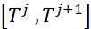
; within the j-th interval, the bias is expressed as a function of temperature and its rate of change:

Where:
 is the equivalent bias at the starting temperature point of segment $j$;
 is the first-order sensitivity coefficient of the bias to temperature within that segment;
 is the sensitivity coefficient of the bias to the rate of temperature change within that segment;
 is the reference temperature.
This model accounts for both steady-state temperature effects (the second term) and dynamic temperature effects (the third term)—the latter being particularly critical during the warm-up phase following startup.
(2) Continuity constraint: the "soul" of piecewise compensation
A critical constraint for piecewise compensation is that the compensation values must be continuous at the boundaries between adjacent temperature segments; otherwise, a sudden jump in the output would occur as the temperature slowly crosses the inflection point, leading to discontinuity in the navigation solution.
The continuity condition can be expressed as:

Upon expansion, the bias of each segment can be expressed recursively in terms of the parameters of the first segment; this allows the fitting parameters for all segments to be treated as a unified whole for least-squares estimation, thereby ensuring the smoothness and continuity of the curve across the entire temperature range.
(3) Inflection Point Identification and Adaptive Segmentation
Segmentation hinges on identifying inflection points—temperature nodes where the slope of the temperature-bias curve changes significantly. An adaptive inflection point identification algorithm is employed in engineering practice, with the following core logic:
a. Reconstruct the bias curve: Subtract the linear baseline (calculated over the full temperature range) from the raw bias data to accentuate the characteristics of the inflection points.
b. Calculate multi-scale slopes: Compute the left and right slopes at intervals of 1°C and 5°C, respectively.
c. Slope sign criterion: Identify temperature points where the signs of the left and right slopes (at the 5°C interval) differ; designate these as candidate inflection points.
d. Validity check: Eliminate "pseudo-inflection points" that are spaced too closely or lack sufficient slope consistency within the interval.
Once inflection points are identified, low-order polynomial fitting (typically second or third-order) is applied within each sub-interval; this approach captures local nonlinearity while avoiding overfitting. The fitting parameters are determined using the least-squares method:

Here, Temp is the temperature matrix, and B represents the corresponding bias observations.
Real-time compensation process
In actual engineering implementation, segmented temperature drift compensation is divided into two stages:
· Offline calibration stage: The IMU is placed in a thermostat to perform temperature cycles across the full temperature range (such as -30°C to 70°C), record the static output at each temperature point, and complete inflection point identification and calculation of fitting parameters for each segment.
· Online compensation stage: The system reads the temperature sensor value in real time, determines the range to which the current temperature belongs, substitutes it into the corresponding model to calculate the compensation amount, and deducts it from the original output:

Research indicates that the adaptive piecewise polynomial method can achieve compensation accuracy comparable to that of the look-up table method while requiring significantly fewer compensation parameters. Regarding system-level heading effect errors caused by temperature fluctuations, a compensation method based on the Fourier expansion of temperature variations can reduce the error by 40% to 90%.
leave a message
Scan to Wechat :