Applications

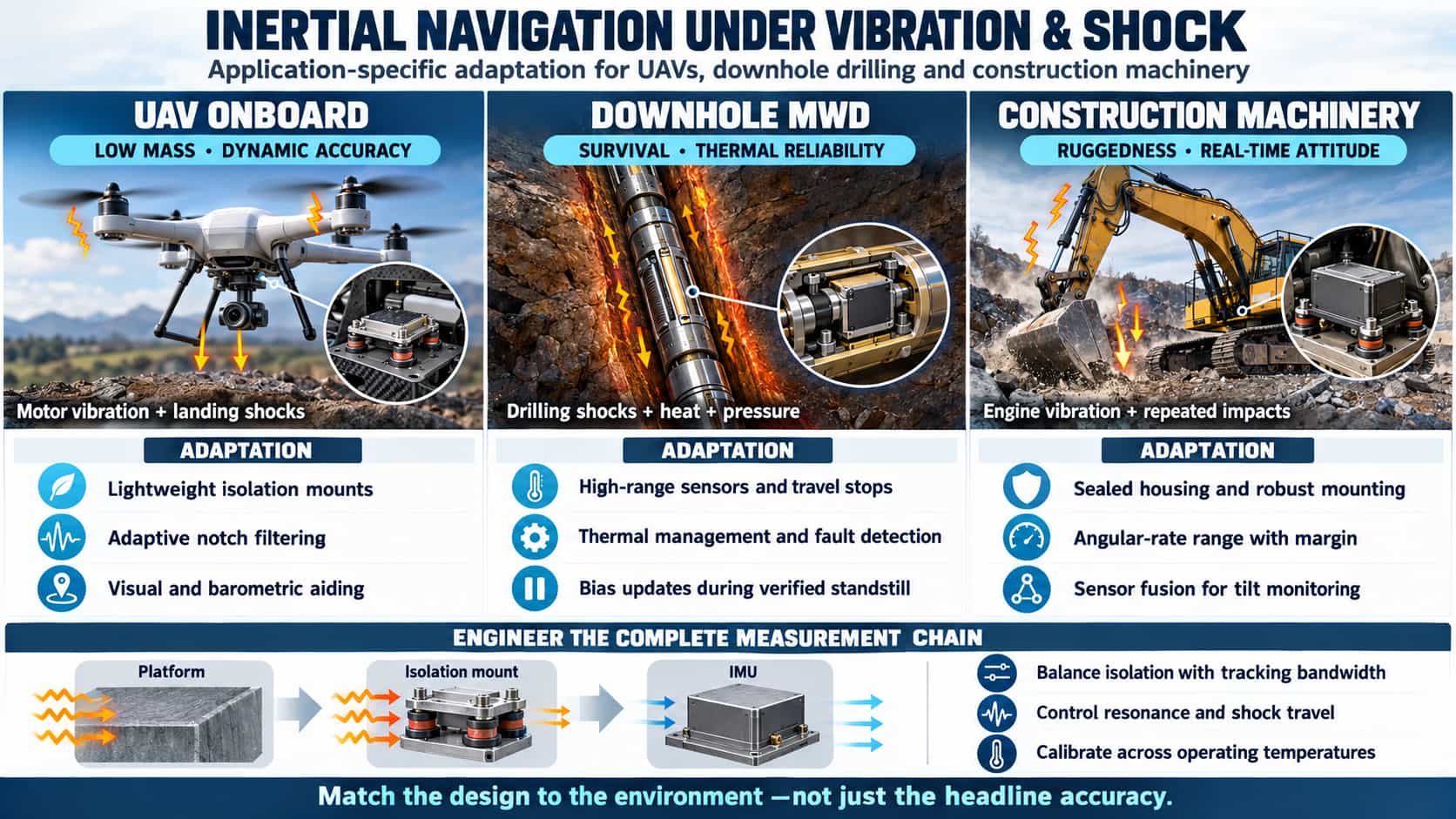
Inertial Navigation Systems (INS), centered on gyroscopes and accelerometers, operate autonomously without relying on external signals to provide continuous navigation data—a capability that offers irreplaceable advantages for unmanned platforms and specialized operational fields. However, as these systems transition from the laboratory to real-world battlefields or operational sites, intense vibration and high-impact forces emerge as the primary factors limiting both their accuracy and service life. While unmanned aerial vehicle (UAV) operations, measurement-while-drilling (MWD) in downhole environments, and the use of heavy construction machinery all fall under the category of "high-impact operating conditions," their specific environmental characteristics and adaptation requirements differ significantly. Understanding these distinctions is a prerequisite for effective, targeted design. 1. Differences in Impact Characteristics and Requirements Across the Three Scenarios In UAV applications, vibrations primarily stem from the high-frequency rotation of motors or engines and the aerodynamic disturbances caused by propellers, resulting in complex, persistent spectral components. Furthermore, the impact of landing, catapult-assisted takeoffs, or the release of mission payloads can induce transient, high-G shocks. For such lightweight platforms, the core requirement for an INS is to maintain dynamic accuracy within strict constraints on size and power consumption, while also balancing cost and ease of integration. Given that UAVs are extremely sensitive to weight, any vibration-damping structure must be implemented within a limited mass budget; excessive reinforcement would otherwise compromise operational endurance. Measurement-while-drilling (MWD) represents the most extreme operational environment. Axial and lateral shocks generated by the drill bit as it breaks through rock can reach levels of 200g to 2000g, accompanied by broadband random vibrations of up to 18grms, all while subjected to temperatures exceeding 150°C and mud pressures of several tens of megapascals. The INS is housed within a drill collar, where space is severely restricted and routine maintenance is impossible. In this context, the priorities for system adaptation are: survivability > high-temperature reliability > measurement accuracy. While some compromise on accuracy may be acceptable, the failure of a sensor would lead to the collapse of drilling operations, potentially resulting in losses of hundreds of thousands of dollars. The vibration characteristics encountered by heavy construction machinery—such as excavators, cranes, mining trucks, and road pavers—fall somewhere between those of the two scenarios described above. Low-frequency engine vibration and impact loads from working implements (such as buckets or booms) serve as the primary sources of excitation. Peak acceleration typically ranges from 10g to 50g—lower than what is encountered in underground mining operations, yet higher than that experienced by standard road vehicles. The operating environment is characterized by frequent, repetitive mechanical motion, drastic changes in orientation, high levels of dust and humidity, and significant temperature fluctuations. In this context, the core function of an inertial navigation system (INS) is to provide a reliable attitude reference and anti-rollover warnings amidst rough, intensive operations; consequently, real-time performance and robustness are prioritized over absolute precision. 2. Differentiated Adaptation Strategies The distinct requirements of these three scenarios dictate specific adaptation strategies for inertial navigation systems: For drone-based applications, the adaptation strategy centers on lightweight vibration isolation and algorithmic compensation. Physically, the IMU module is decoupled from the airframe using miniature elastic damping materials, with the natural frequency of the isolators carefully selected to avoid the primary operating frequencies (and their harmonics) of the motors. Algorithmically, the system leverages existing acceleration feedback from the drone’s flight controller to identify dominant vibration frequencies in real-time, employing adaptive notch filters to suppress interference. Recent approaches have also explored the "tight coupling" of the IMU with multi-source sensors—such as vision systems and barometers—using visual features to provide attitude constraints during periods of intense vibration, thereby reducing reliance on pure inertial navigation. For underground "while-drilling" applications, the focus shifts to hardware hardening and redundancy-based fault tolerance. Accelerometers and gyroscopes must feature high-range, closed-loop architectures and incorporate mechanical limit stops to withstand extreme impacts. To manage high temperatures, the enclosure utilizes a thermal management strategy that combines insulation layers with dedicated heat-conduction paths. At the system level, a triple-redundant IMU configuration is standard; if one sensor produces an anomalous output due to an impact, the system automatically isolates the faulty channel via majority voting or residual monitoring mechanisms. Furthermore, these systems employ "zero-velocity updates" (ZUPT)—calibrating sensor bias during the static intervals when drilling is paused to add a new drill pipe, which effectively mitigates cumulative drift caused by vibration. For construction machinery, the adaptation strategy prioritizes environmental protection and operational adaptability. An IP67 or higher ingress protection rating is the baseline requirement to withstand dust exposure and high-pressure water washdowns. Given the intense angular motion triggered by the extension and retraction of booms during operation, the gyroscope’s measurement range must include a sufficient safety margin (typically selecting a range of at least ±300°/s). To counter the degradation of zero-point stability caused by frequent impacts, the system should incorporate an automatic zero-calibration routine, refreshing the bias during brief operational windows—such as when the engine is idling or the working equipment is stationary. Furthermore, inertial navigation outputs are commonly fused with data from GNSS receivers and inclinometers to form a safety monitoring system; this triggers an immediate alert if the vehicle’s tilt exceeds a defined threshold, thereby preventing rollovers. 3. General Design Principles Despite the diversity of operational environments, the adaptation of inertial navigation systems across these three categories follows several common principles: physical isolation takes precedence over algorithmic correction—structural vibration damping serves as the primary line of defense, and algorithmic compensation is only truly effective when built upon such a foundation. A trade-off between measurement range and accuracy is necessary; sensors with higher ranges often sacrifice resolution and zero-bias stability, so selection must balance the relative importance of peak impact tolerance against navigation precision. Additionally, full-temperature-range calibration is essential—since the combined effects of vibration and high temperatures significantly alter a sensor’s error model compared to room-temperature conditions, factory calibration must encompass the entire expected operating temperature range. Conclusion While drones prioritize being "lightweight and precise," underground mining equipment demands "ruggedness and stability," and construction machinery requires "durability and practicality." Adapting inertial navigation systems for these high-impact environments is, at its core, a quest for the optimal balance between accuracy, survivability, size/power consumption, and cost. As MEMS technology continues to evolve—pushing toward both higher measurement ranges and lower noise levels—and as multi-source fusion navigation algorithms mature, a new paradigm is likely to emerge: standardized IMU hardware paired with application-specific software. This approach promises to meet the increasingly diverse requirements of high-impact operating environments at a lower cost.

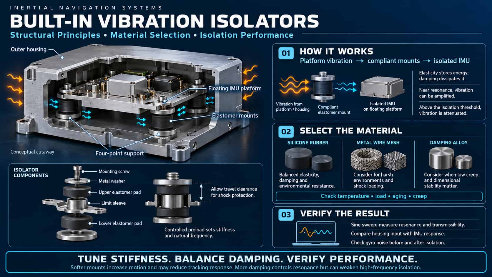
Introduction   The core components of an Inertial Navigation System (INS)—gyroscopes and accelerometers—are highly sensitive to the vibration environment of the host platform. Vibration can induce additional drift in gyroscopes and increase output errors in accelerometers; in severe cases, it may even cause the entire system to fail. Consequently, the integration of vibration isolators has become an essential aspect of INS design. Their primary function is to establish physical isolation between the platform’s vibrations and the inertial sensors, effectively attenuating high-frequency vibrations to ensure that the INS continues to provide high-precision navigation data, even under complex operating conditions.   Structure and Principles of Vibration Isolators   Basic Configuration   An INS vibration isolator is essentially a spring-damper unit. Taking the common four-point mounting configuration as an example, each isolator consists of the following components: Rubber damping pads (one on top and one on the bottom): These provide elasticity and damping, serving as the core elements for vibration isolation. Metal limiting sleeves: These constrain the compression of the rubber pads, preventing damage from overloading. Metal shims: These transmit fastening force and work in conjunction with the limiting sleeves to control the degree of pre-compression. Mounting screws: These secure the entire assembly to the mounting surface of the host platform. During installation, as the screws are tightened, the metal shims move downward until they reach the limiting shoulder, inducing a controlled amount of pre-compression in the upper and lower rubber damping pads. This level of compression directly influences the stiffness and natural frequency of the isolator, making it a critical process parameter for performance control.   Mechanical Model   A single vibration isolator can be simplified as a single-degree-of-freedom (SDOF) spring-damper-mass system, the vibration transmission characteristics of which can be described by a transmissibility coefficient, η: Where: "A_transfer" is the vibration amplitude transmitted to the device; "A_external" is the amplitude of the external excitation vibration. λ = ω/ω_n: Frequency ratio, where ω is the excitation frequency and ω_n is the natural frequency of the system. ξ = c/(2√mk): Damping ratio, where c is the damping coefficient, k is the stiffness, and m is the mass. When λ ≈ 1, the system enters resonance, and the transmissibility η reaches a peak value of η_max ≈ 1/(2ξ); in this state, vibration is amplified rather than attenuated. When λ > √2, η < 1, and the vibration isolator enters the effective isolation range; a larger λ results in better isolation performance. Beyond λ > 5, the rate of attenuation levels off; in engineering practice, λ is typically selected in the range of 2.5 to 4.5. Vibration isolation efficiency α is defined as: α = (1 - η) × 100%.   Design Objectives   The design of an inertial navigation system (INS) vibration isolation system must meet the following requirements: The natural frequency ω_n is typically designed to be between 50–60 Hz, ensuring that the low-frequency vibrations of the carrier (2–200 Hz) fall within the effective isolation range. A damping ratio ξ of approximately 0.1 (corresponding to a loss factor β ≈ 0.2) is chosen to balance the suppression of resonance peaks with efficiency in the isolation range. Equal stiffness in all three axes (X, Y, and Z) is required to ensure balanced isolation performance across these directions and to prevent angular vibration coupling. Taking a vehicle-mounted inertial navigation system as an example: by selecting a frequency ratio λ = 2.5 and an isolation frequency of 150 Hz, the resulting natural frequency f_n is 60 Hz, with a damping ratio ξ = 0.10, a transmissibility η = 0.195, and a vibration isolation efficiency α = 80.5%.   Material Selection   Comparison of Common Materials Materials for inertial navigation vibration isolators must balance four key factors: elasticity, damping, environmental adaptability, and service life. Mainstream solutions include: Selection Principles   For standard airborne or vehicle-mounted inertial navigation systems (INS), silicone rubber is the preferred choice. It offers distinct advantages, including high damping, stability across a wide temperature range, and a long service life; for instance, the domestically produced SE-series silicone rubber vibration isolators can achieve a vibration isolation efficiency of over 90%. For extreme environments—such as those encountered in space or involving rapid, high-to-low temperature cycling—metal rubber or damping alloys are more suitable. The inertial navigation system of the Mars rover, for example, utilizes metal rubber vibration isolators capable of operating across a temperature range of -50°C to 75°C, while providing over 80% attenuation against shocks exceeding 1,000 G. For high-precision attitude measurement applications, damping alloys are superior to rubber; their high stiffness and minimal creep prevent deformation of attitude angles (maintaining an error of less than 30 arcseconds).   Optimization Strategy   Research and practical experience indicate that, while maintaining necessary structural strength, one should select rubber materials with a lower Shore hardness. Additionally, increasing the height of the damping pad and the difference between its inner and outer diameters helps lower the natural frequency and enhance vibration-damping efficiency.   Verification of Vibration-Damping Performance   The vibration-damping performance for inertial navigation systems (INS) is verified through sinusoidal sweep vibration testing. By analyzing the resulting amplitude-frequency characteristic curves (transmissibility vs. frequency), the following are evaluated: Whether the resonant frequency lies outside the operational frequency range. Whether the resonant amplification factor meets specified requirements (typically < 5–6 dB). Whether the -3 dB bandwidth covers the target frequency range for vibration isolation.   Experimental results for an INS vibration-damping system in a drone showed a resonant frequency of 55 Hz, a maximum acceleration transmissibility of 2.2 (approximately 6.8 dB), and a -3 dB bandwidth of 30–40 Hz—all meeting the design specifications. Following the implementation of the damping system, the standard deviation of the gyroscope output was reduced to 34.6%–43.5% of its original value, confirming the system's effectiveness.   Conclusion   Built-in INS vibration dampers utilize a spring-damping mechanism to effectively attenuate vibrations from the host platform along the transmission path. The core of the design lies in the optimal balancing of the natural frequency and damping ratio, ensuring that the operational frequency range falls within the vibration-isolation zone (where the transmissibility ratio $\lambda > \sqrt{2}$) while simultaneously suppressing resonant peaks. In terms of materials, silicone rubber is the mainstream choice due to its comprehensive advantages, whereas metal rubber and damping alloys serve indispensable roles in extreme environments. A well-designed vibration-damping system can attenuate vibration interference by 70%–90%, providing a robust mechanical foundation for high-precision output from inertial navigation systems.

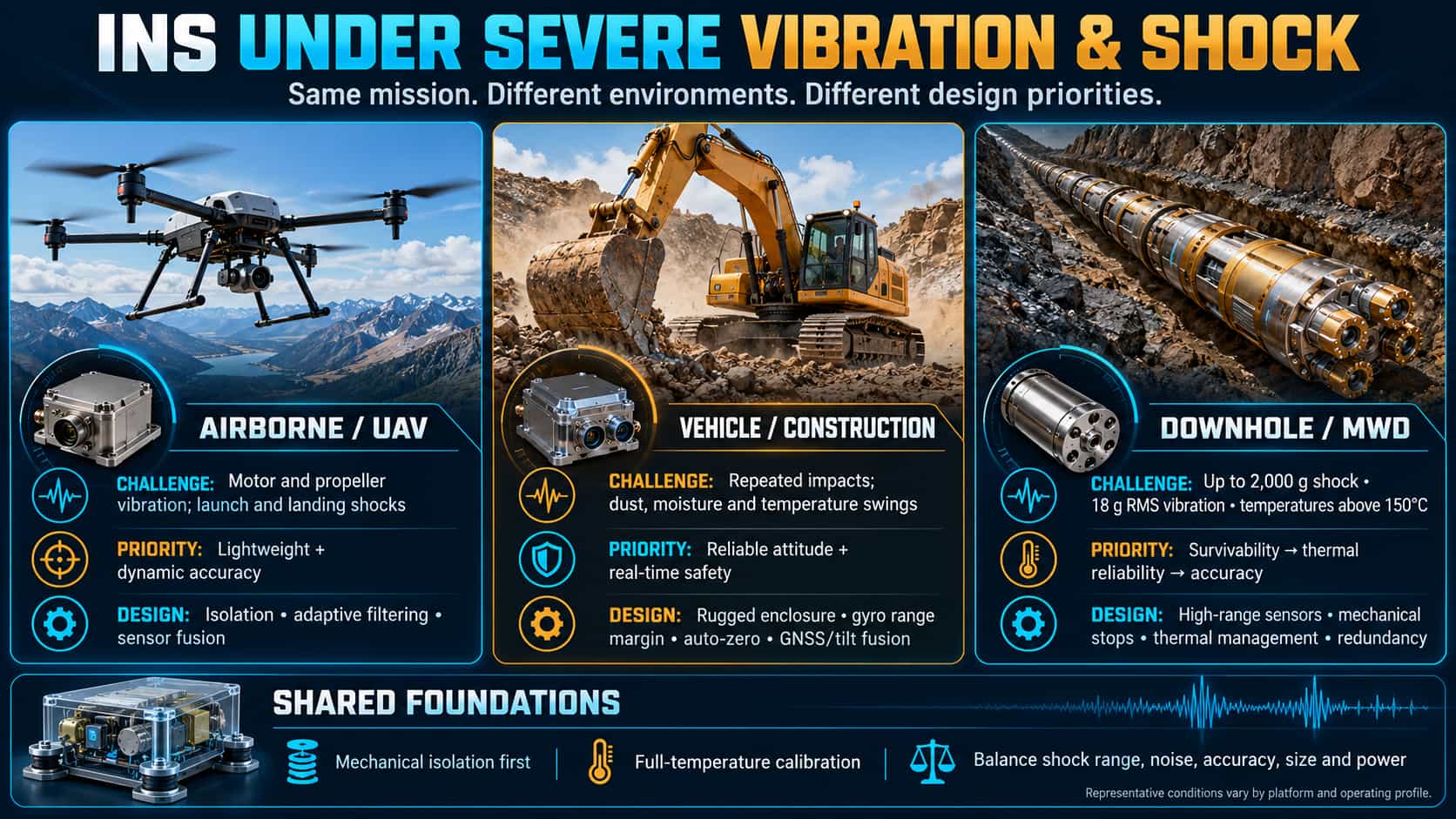
Inertial Navigation Systems (INS), centered on gyroscopes and accelerometers, operate autonomously without relying on external signals to provide continuous navigation data—a capability that offers irreplaceable advantages for unmanned platforms and specialized operational fields. However, as these systems transition from the laboratory to real-world battlefields or operational sites, intense vibration and high-impact forces emerge as the primary factors limiting both their accuracy and service life. While unmanned aerial vehicle (UAV) operations, measurement-while-drilling (MWD) in downhole environments, and the use of heavy construction machinery all fall under the category of "high-impact operating conditions," their specific environmental characteristics and adaptation requirements differ significantly. Understanding these distinctions is a prerequisite for effective, targeted design. 1. Differences in Impact Characteristics and Requirements Across the Three Scenarios In UAV applications, vibrations primarily stem from the high-frequency rotation of motors or engines and the aerodynamic disturbances caused by propellers, resulting in complex, persistent spectral components. Furthermore, the impact of landing, catapult-assisted takeoffs, or the release of mission payloads can induce transient, high-G shocks. For such lightweight platforms, the core requirement for an INS is to maintain dynamic accuracy within strict constraints on size and power consumption, while also balancing cost and ease of integration. Given that UAVs are extremely sensitive to weight, any vibration-damping structure must be implemented within a limited mass budget; excessive reinforcement would otherwise compromise operational endurance. Measurement-while-drilling (MWD) represents the most extreme operational environment. Axial and lateral shocks generated by the drill bit as it breaks through rock can reach levels of 200g to 2000g, accompanied by broadband random vibrations of up to 18grms, all while subjected to temperatures exceeding 150°C and mud pressures of several tens of megapascals. The INS is housed within a drill collar, where space is severely restricted and routine maintenance is impossible. In this context, the priorities for system adaptation are: survivability > high-temperature reliability > measurement accuracy. While some compromise on accuracy may be acceptable, the failure of a sensor would lead to the collapse of drilling operations, potentially resulting in losses of hundreds of thousands of dollars. The vibration characteristics encountered by heavy construction machinery—such as excavators, cranes, mining trucks, and road pavers—fall somewhere between those of the two scenarios described above. Low-frequency engine vibration and impact loads from working implements (such as buckets or booms) serve as the primary sources of excitation. Peak acceleration typically ranges from 10g to 50g—lower than what is encountered in underground mining operations, yet higher than that experienced by standard road vehicles. The operating environment is characterized by frequent, repetitive mechanical movements, drastic changes in orientation, high levels of dust and humidity, and significant temperature fluctuations. In this context, the core function of an inertial navigation system (INS) is to provide a reliable attitude reference and anti-rollover warnings amidst rough, intensive operations; consequently, real-time performance and robustness are prioritized over absolute precision. 2. Differentiated Adaptation Strategies The distinct requirements of these three scenarios dictate specific adaptation strategies for inertial navigation systems: For drone-based applications, the adaptation strategy focuses on lightweight vibration isolation and algorithmic compensation. Physically, the IMU module is isolated from the airframe using miniature elastic damping materials, with the natural frequency of the isolators carefully selected to avoid the primary operating frequencies (and their harmonics) of the motors. Algorithmically, the system leverages acceleration feedback from the drone’s flight controller to identify dominant vibration frequencies in real time, employing adaptive notch filters to suppress interference. Recent approaches have also explored the "tight coupling" of the IMU with other sensors—such as vision systems and barometers—using visual features to provide attitude constraints during periods of intense vibration, thereby reducing reliance on the accuracy of pure inertial navigation. For underground "while-drilling" applications, the focus shifts to hardware hardening and redundancy-based fault tolerance. Accelerometers and gyroscopes must feature high-range, closed-loop architectures and incorporate mechanical limit stops to withstand extreme impacts. To manage high temperatures, the enclosure utilizes a thermal management strategy that combines insulation layers with dedicated heat-conduction paths. At the system level, a triple-redundant IMU configuration is standard; if one sensor produces anomalous output due to an impact, the system automatically isolates the faulty channel via majority voting or residual monitoring mechanisms. Furthermore, these systems employ "zero-velocity updates" (ZUPT)—calibrating sensor bias during the brief pauses in drilling (such as when adding a new drill pipe) to effectively mitigate cumulative drift caused by vibration. For construction machinery, the adaptation strategy prioritizes environmental protection and operational adaptability. An IP67 or higher ingress protection rating is the baseline requirement to withstand dust exposure and high-pressure water washdowns. Given the intense angular motion triggered by the extension and retraction of booms during operation, the gyroscope’s measurement range must include a sufficient safety margin (typically selecting a range of at least ±300°/s). To counter the degradation of zero-point stability caused by frequent impacts, the system should incorporate an automatic zero-calibration routine, refreshing the bias during brief operational windows—such as when the engine is idling or the working equipment is stationary. Furthermore, inertial navigation outputs are commonly fused with data from GNSS receivers and inclinometers to establish a safety monitoring system; this triggers an immediate alert if the vehicle’s tilt exceeds a defined threshold, thereby preventing rollovers. 3. General Design Principles Despite the diversity of operational environments, the adaptation of inertial navigation systems across these three categories follows several common principles: physical isolation takes precedence over algorithmic correction—structural vibration damping serves as the primary line of defense, and algorithmic compensation can only be effective when built upon such a foundation. A trade-off between measurement range and accuracy is necessary; sensors with higher ranges often sacrifice some resolution and zero-bias stability, so selection must balance the relative importance of peak impact tolerance against navigation precision. Additionally, full-temperature-range calibration is essential; because the combined effects of vibration and high temperatures significantly alter a sensor’s error model compared to room-temperature conditions, factory calibration must encompass the entire expected operating temperature range. Conclusion While drones prioritize being "lightweight and precise," underground equipment demands "ruggedness and stability," and construction machinery requires "durability and practicality." Adapting inertial navigation systems for these high-impact environments is, at its core, a quest for the optimal balance between accuracy, survivability, size/power consumption, and cost. As MEMS technology continues to evolve—pushing toward both higher measurement ranges and lower noise levels—and as multi-source fusion navigation algorithms mature, a new paradigm is likely to emerge: standardized IMU hardware paired with application-specific software. This approach promises to meet the requirements of increasingly diverse, high-impact operational scenarios at a lower cost.

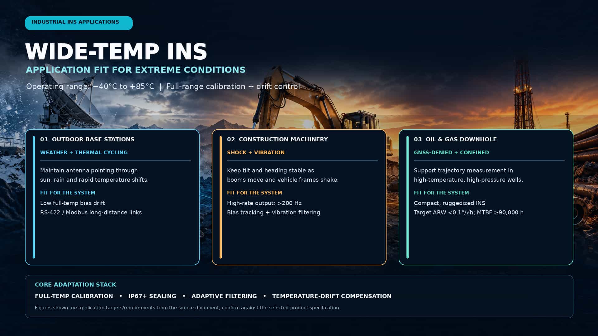
Automated and high-precision operations for outdoor base stations (e.g., satellite communication antennas), construction machinery (e.g., excavators, AGVs), and downhole oil and gas equipment (e.g., logging tools) rely heavily on stable, reliable attitude sensing and navigation/positioning capabilities. However, these applications often face extreme environmental challenges, including wide operating temperature ranges (-40°C to +85°C), intense vibration, high shock loads, high humidity, and electromagnetic interference. Conventional inertial navigation products are prone to issues such as bias drift and nonlinear scale factor variations in these environments, leading to reduced measurement accuracy. Consequently, inertial navigation products must be rigorously adapted across three dimensions—hardware selection, temperature compensation, and algorithmic interference rejection—to meet the stringent requirements of industrial-grade applications. Core Hardware Selection: Wide Temperature Range and Environmental Protection Hardware serves as the first line of defense against environmental interference. For harsh operating conditions, hardware selection for inertial navigation products must prioritize the following characteristics: Wide-Temperature Operation and Full-Range Calibration: Products must support an operating temperature range of -40°C to +85°C. Simply using wide-temperature components is insufficient to guarantee accuracy; system-level calibration across the entire temperature range is essential. By establishing full-temperature parameter models (e.g., temperature coefficients for bias and scale factor) for MEMS gyroscopes and accelerometers and applying compensation, error divergence in environments with significant temperature fluctuations can be significantly mitigated. For instance, certain high-specification IMUs can maintain bias stability within 0.1°/s across the entire temperature range. High Mechanical Strength and Sealing: Construction machinery and downhole equipment are often subjected to shocks of up to 20,000g and vibrations of 10grms. Inertial navigation housings must utilize high-strength materials—such as magnesium-aluminum alloys—and feature sealing designs rated IP67 or higher to prevent the ingress of dust and liquids. Additionally, internal structural optimization is required to minimize the impact of assembly stress on sensor performance. Core Algorithmic Strategies: Thermal Drift Suppression and Vibration-Resistant Filtering Hardware determines the baseline performance, while algorithms determine the performance ceiling. For wide-temperature operating environments, algorithmic adaptation strategies include: (1) High-precision temperature drift compensation algorithms: Relying solely on hardware-based temperature compensation (such as thermistor-based methods) is often insufficient to meet high-precision requirements. Current mainstream approaches employ data-driven modeling techniques—such as using Fourier series expansions to characterize the impact of temperature fluctuations on heading, or utilizing Particle Swarm Optimization (PSO) to identify temperature-error models—to achieve precise compensation for zero-bias drift. Literature indicates that such integrated compensation techniques can reduce temperature-induced heading errors by 40% to 90%. (2) Adaptive filtering and anti-vibration techniques: Environments with intense vibration introduce high-frequency noise, leading to angular rate random walk and the accumulation of velocity errors. By implementing adaptive filtering and resonance suppression techniques (e.g., notch filters), it is possible to effectively distinguish between actual motion and interfering vibrations, thereby mitigating the impact of noise on integrated attitude solutions. Furthermore, by combining these methods with Kalman filtering and utilizing accelerometer and magnetometer data for the online correction of gyroscope drift, attitude accuracy can be maintained during brief periods of GNSS denial or signal loss. Analysis of adaptation for typical application scenarios In summary, inertial navigation products designed for wide-temperature environments—such as outdoor base stations, construction machinery, and oil wells—are far more than a mere assembly of components. Their technical core lies in hardware ruggedness, temperature-resilient algorithms, and system-level interference immunity. The key to achieving highly reliable, long-lasting industrial inertial navigation lies in utilizing automotive- or industrial-grade wide-temperature MEMS chips, performing precise calibration and compensation across the full temperature range prior to shipment, and incorporating advanced filtering algorithms optimized for vibration and thermal drift.

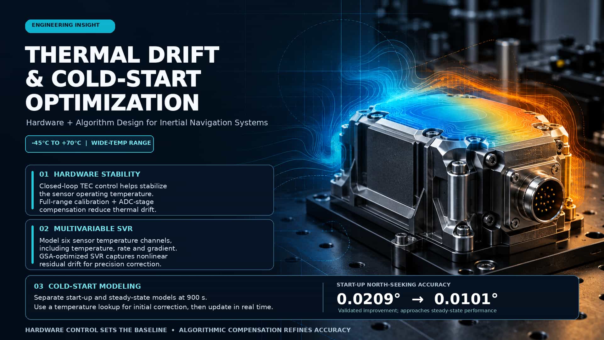
The accuracy of inertial navigation systems is significantly constrained by temperature effects. Under wide operating temperature ranges (e.g., -45°C to +70°C), the bias and scale factor of inertial components (gyroscopes and accelerometers) exhibit significant drift; errors associated with high-temperature drift and the low-temperature startup phase are particularly pronounced. High-temperature drift stems from changes in material properties as temperature rises, whereas low-temperature startup involves transient heat transfer effects during the establishment of the internal thermal field. To address these two critical issues, this paper systematically outlines optimization design methods from both hardware and algorithmic perspectives. 1. High-Temperature Drift: Mechanism Analysis and Hardware-Algorithm Co-optimization 1.1. Drift Mechanism In high-temperature environments, drift in inertial components primarily arises from the temperature sensitivity of the materials. Taking silicon-based MEMS devices as an example, the relationship between the elastic modulus and temperature can be approximately expressed as: ； The temperature coefficient of the elastic modulus of silicon material. This change directly causes a shift in the resonant frequency: For a laser gyro, the relative error in the scale factor caused by the variation of the resonant cavity length with temperature is: In the formula, ρ represents the coefficient of thermal expansion. Taking a glass-ceramic resonant cavity as an example, where ρ = 5.5 × 10⁻⁷/°C, a temperature change of 110°C introduces an error of approximately 60 ppm. 1.2 Hardware Optimization Strategies Thermal Control Architecture Design: A closed-loop thermal control system is established using a thermally insulated housing combined with a thermoelectric cooler (TEC) to maintain the operating zone of the inertial components at a near-constant temperature. Temperature sensors monitor the ambient temperature in real time, while the MCU regulates the direction and magnitude of the TEC current via a current controller, enabling dual-mode control for both heating and cooling. Full-Temperature-Range Calibration and Hardware Compensation: A temperature compensation mechanism is incorporated into the analog-to-digital conversion stage. For high-precision I/F conversion circuits, a model correlating the circuit's intrinsic zero-offset output with the temperature field is established under zero-input-current conditions; subsequently, secondary compensation is applied to the acceleration channel as a whole to prevent mismatches between independent compensation efforts and the system's thermal environment. 1.3 Algorithmic Compensation Methods Multivariate Temperature Field Modeling: A single thermometer cannot fully capture the complex temperature field distribution within the inertial navigation unit. The optimal approach utilizes data from the built-in thermometers of six inertial sensors to construct multidimensional temperature variables—specifically temperature ($T$), rate of temperature change ($\dot{T}$), and temperature gradient ($\nabla T$)—which serve as inputs for the compensation model. Support Vector Regression (SVR) Modeling: Thermal drift in inertial components exhibits strong nonlinearity, rendering traditional polynomial fitting insufficiently accurate. SVR achieves nonlinear regression by mapping data into a high-dimensional feature space using kernel functions. The regression function is expressed as: Select the radial basis kernel function： The kernel parameter σ and the penalty factor C significantly affect model accuracy, necessitating the use of meta-heuristic algorithms (such as the Gravitational Search Algorithm, GSA) for optimization. Experimental results demonstrate that the GSA-SVR-based compensation method can improve navigation accuracy by more than 50%. 2. Cold Start: Segmented Modeling of Startup and Steady-State Phases Cold start represents one of the most rigorous challenges for inertial navigation products. Upon initial power-up, the system's internal temperature field has not yet stabilized; differences in thermal inertia among components lead to non-uniform transient temperature rises, causing drift errors to exhibit non-stationary characteristics. The key approach is to model the startup phase (typically the first 20 minutes) and the steady-state operation phase separately. 2.1 Error Characteristics During the Startup Phase During a cold start, the resonant drive has not yet stabilized and the circuitry is in a warm-up state; temperature fluctuations stem primarily from heat generated by the components themselves. The magnitude of output drift during the gyroscope's startup phase is often several times greater than that observed during the steady-state phase. An initial error compensation value, $C(T_0)$, is obtained via a lookup table based on the temperature $T_0$ detected at the moment of startup to provide immediate compensation, which is then updated in real-time during subsequent operation. 2.2 Segmented Compensation Algorithm An SVR (Support Vector Regression) scheme based on segmented modeling is employed: operational states are categorized based on the time elapsed since power-up (typically using a 900-second threshold), and separate temperature drift models are trained for the startup and steady-state phases. This strategy has been validated in fiber-optic gyro north-seeking instruments, where the accuracy during the startup phase improved from 0.0209° to 0.0101°, approaching the performance level of the steady-state phase. The recursive form of the temperature error compensation can be expressed as follows: Here, is the initial look-up table value at the start time, is the temperature difference between consecutive sampling instants, and are the error coefficients for the rate of temperature change and its quadratic term, respectively. Conclusion The issues of high-temperature drift and low-temperature startup in inertial navigation products are fundamentally manifestations of the interplay between material temperature sensitivity and thermal field non-uniformity. Engineering practice demonstrates that a synergistic strategy—using hardware thermal control to establish a baseline and algorithmic compensation to further enhance performance—is the most effective approach: at the hardware level, TEC-based thermal control and full-temperature-range calibration are employed to suppress the magnitude of drift, while at the algorithmic level, piecewise SVR multivariate modeling is used for refined residual compensation. Combining these methods effectively reduces startup time and improves accuracy across the entire operating temperature range of -45°C to +70°C.

As unmanned systems evolve toward higher speed, greater maneuverability, and stronger autonomy, the bottleneck in motion control systems often lies not in algorithms but in whether front-end inertial sensors can promptly and accurately sense high angular rates. Conventional MEMS gyroscopes are prone to entering saturation or exhibiting noticeable delay during sharp turns of high-speed UAVs, off-road driving of unmanned combat vehicles, or rapid joint movements of robots. To meet these needs, the MG series ultra-wide-range MEMS gyroscopes developed by Micro-Magic Inc. extend the measurement range from ±100°/s to ±10800°/s and position ±4000°/s-class products as the primary measurement range for high-speed motion control. The core idea behind this series is not merely to pursue a wide range, but to maintain the dynamic quality required for closed-loop control across a wide range. The MG series adopts a 24-bit resolution architecture, with a maximum data output rate of up to 12kHz, group delay below 1.5 ms in most high-range models, and bandwidth above 180Hz. For ±4000°/s-class models, such as the MG-4001, bias instability is below 0.3°/h, angular random walk is below 0.25°/√h,  broadband noise peak-to-peak is below 1°/s, and both g-sensitivity and vibration rectification error are below 1°/h/g. These specifications mean that the sensor can still provide angular rate information usable for attitude determination and stabilization control in rapid maneuvering and vibration environments. Environmental adaptability is another unavoidable dimension for unmanned platforms. The MG series supports an operating temperature range of -40°C ~ +85°C. Its vibration resistance reaches 18 grms, and its shock resistance is up to 500g/1ms. 5V supply and typical current consumption of 45 mA also make the series easy to integrate into unmanned systems with strict requirements on power consumption and power supply architecture. 750ms startup time makes it suitable for mission scenarios requiring rapid power-on readiness. The MG series is not a single model, but a family spanning multiple measurement ranges and accuracy grades. The low-range MG-101 and MG-102 target high-precision attitude measurement; mid-range models such as the MG-301 and MG-401 balance range and stability, making them suitable for general unmanned platforms; and the high-range MG-4001, MG-8001, and MG-10800 push the upper measurement limit to ±4000°/s, ±8000°/s, and ±10800°/s, respectively, offering options for high-speed rotation, high maneuverability, and extreme angular rate scenarios. This scalability enables designers to match sensors to actual motion profiles instead of making excessive compromises among range, accuracy, and cost. The value of the MG series lies in combining the two requirements of "wide range" and "suitability for control" in a single MEMS gyroscope. It is neither a coarse sensor that pursues range alone nor a high-precision device that can only operate at low speeds. As unmanned systems continue to evolve toward higher speed and greater autonomy, MEMS gyroscopes like the MG series - covering ranges of ±4000°/s and above while maintaining low latency, high bandwidth, and strong environmental adaptability - are becoming key foundational components for breaking through the bottleneck in high-speed motion control.

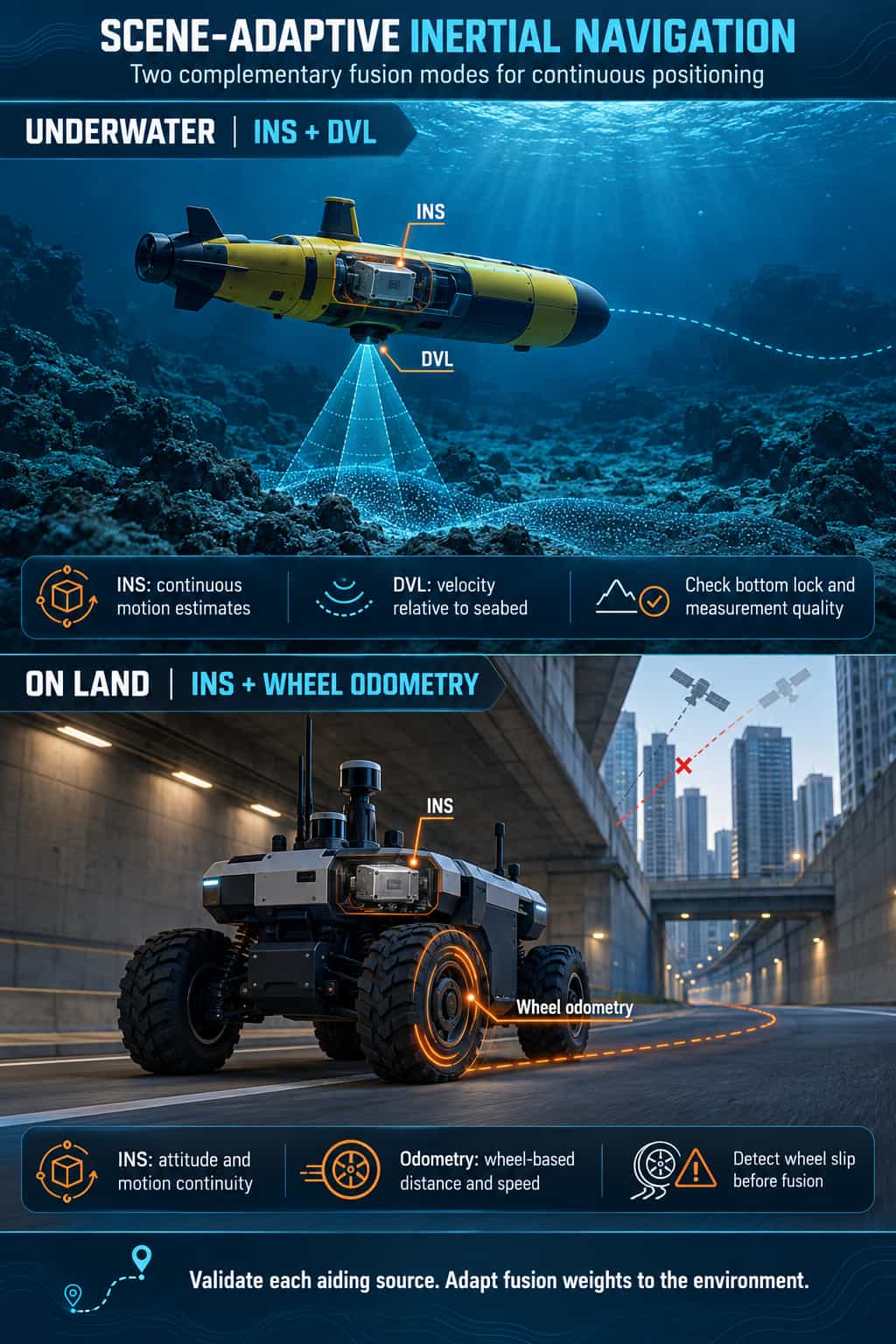
The accumulation of error over time is an inherent limitation of Inertial Navigation Systems (INS), typically necessitating correction via external sensors. Underwater, Doppler Velocity Logs (DVL) provide velocity observations, while on land, odometers (OD) facilitate dead reckoning. Although these approaches appear distinct, they are unified under the mathematical framework of "kinematic constraint-aided filtering." This paper provides an in-depth comparison of the technical characteristics of INS/DVL and INS/OD navigation systems, focusing on their error models and Kalman filter fusion strategies, while revealing how environmental factors—specifically "ocean current disturbances" in underwater settings and "anomalous measurements" in land-based environments—have driven divergent algorithmic evolutions. From "Pure Inertial" to "Observation Fusion" With its autonomous operation, an inertial navigation system (INS) plays a central role in GPS denied environments, such as underwater locations and tunnels. However, its navigation errors grow through integration. Let the velocity computed by the INS be vins and the true velocity be v. The velocity error δv =vins− v satisfies the following equation: δ= f×∅+∇ Here, f is the specific force, ∅ is the misalignment angle, and ∇ is the accelerometer bias. Introducing an external aiding source is the only way to suppress this error. Underwater, a DVL is commonly used to obtain the vehicle’s velocity relative to the ground; on land, an odometer is commonly used to obtain its forward velocity. The state equations of the two systems are largely identical, with the main differences lying in the formulation of their measurement equations and their noise characteristics. A Unified Fusion Framework Based on the Error State Kalman Filter Both underwater and land based integrated navigation systems commonly use an error state Kalman filter (ESKF). The system state vector x generally includes the velocity error δvn, attitude misalignment angle ∅, position error δp, and the biases b and scale factor errors s of the inertial sensors. The state equation takes the following unified form: = Fx + Gw At the measurement level, both systems share the same objective: to construct the measurement equation z = Hx + v from the difference between the external sensor measurement zaux and the INS predicted value zins. Underwater INS DVL Navigation Using Velocity Observations A DVL uses the acoustic Doppler effect to measure the vehicle’s three dimensional velocity in its own coordinate frame. After this velocity is transformed into the navigation frame (n frame) and compared with the INS velocity, the measurement equation is: 最小化图片 编辑图片 删除图片 This measurement equation is straightforward. However, when the DVL is affected by ocean currents or loses beam lock, its measurement noise vdvl may be accompanied by severe outliers. Land Based INS Odometer Navigation Using Velocity and Motion Constraints The motion of a land vehicle is subject to nonholonomic constraints (NHC), meaning that it has no lateral slip or vertical jumping motion. Although the odometer provides only the forward velocity vod, these constraints can be used to construct a three dimensional velocity observation. Let the odometer output in the vehicle body frame be =[0 , 0 ,vod]T. The measurement equation is then: 最小化图片 编辑图片 删除图片 In addition, the odometer scale factor error sod is a key state variable that must be estimated in real time within the filter or calibrated offline. Core Challenges and Diverging Algorithms Under Environmental Constraints Underwater ocean currents introduce unknown biases into DVL measurements, so an interacting multiple model (IMM) approach uses soft switching to adapt to the environment. On land, tire slip causes abrupt changes in odometer measurements, so robust filtering adaptively inflates the noise covariance to reduce the impact of anomalies. These approaches use multiple models and robust estimation, respectively, to address persistent uncertainty and sudden disturbances, reflecting the fundamental constraints that the environment imposes on algorithm design. Underwater Navigation Using IMM to Address Ocean Currents In the presence of ocean currents, a condition described as “stationary on the seabed” appears as constant velocity motion in the navigation frame, causing conventional zero velocity updates (ZUPT) to fail. An IMM aided ZUPT method has been proposed to address this problem. The IMM algorithm runs several models in parallel, such as an INS/DVL model and an INS/ZUPT model, and uses model probabilities for soft switching. When the vehicle’s velocity relative to the water is very small, the weight of the ZUPT model increases, effectively suppressing DVL errors. When appreciable ocean currents are present, the algorithm switches back to the INS/DVL model. Land Navigation Using Robust Filtering to Address Wheel Slip A critical limitation of odometers is the mismatch between wheel derived velocity and ground velocity during wheel slip. In this case, vod in the measurement equation contains large errors and no longer satisfies the Gaussian white noise assumption. The response is to introduce robust estimation. By constructing an equivalent weighting function or reformulating the measurement noise covariance matrix R, the filter automatically inflates R when an abnormally large innovation k is detected, reducing the influence of the anomalous measurement on the filter estimate. Conclusion Underwater INS/DVL navigation and land based INS/odometer navigation are, in mathematical terms, both velocity observation fusion problems based on an error state Kalman filter. Their central difference lies in the sources of error: underwater, complex ocean currents invalidate the constraints; on land, nonideal road conditions cause abrupt changes in measurements. This difference leads to distinct algorithmic strategies. Underwater navigation relies more heavily on multiple model soft switching (IMM) to adapt to unknown hydrodynamic conditions, whereas land navigation relies more heavily on robust estimation within a single model to resist sudden measurement anomalies. Understanding this shared mathematical structure and its different error sources is essential to designing highly reliable and robust integrated navigation systems.  

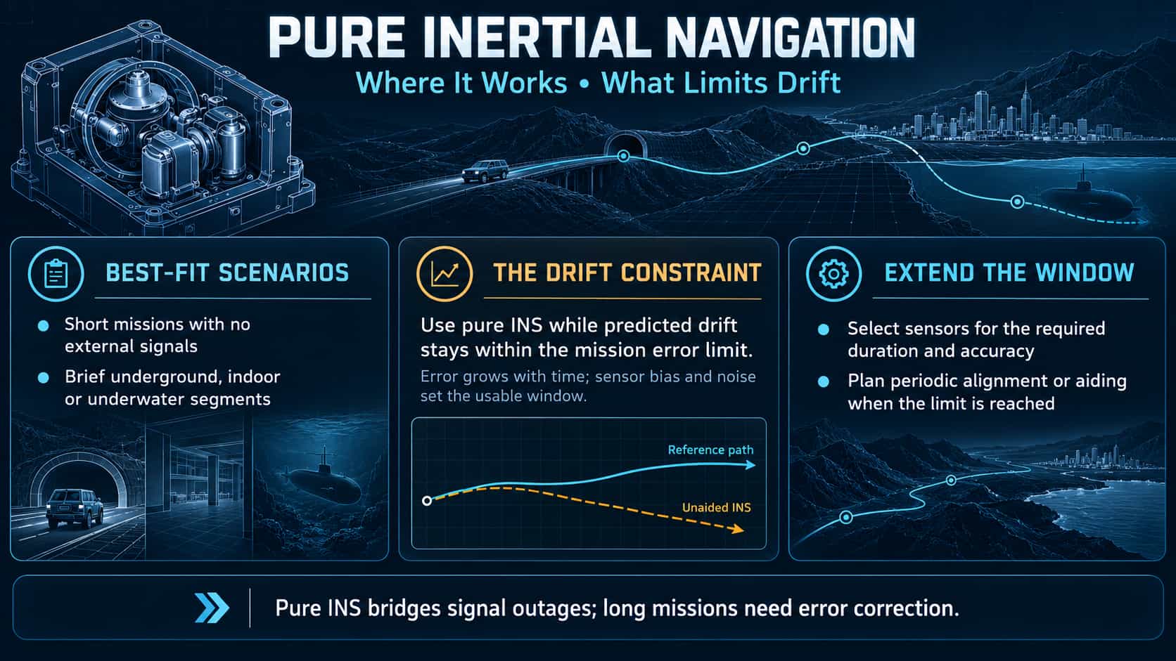
A pure inertial navigation system (INS) relies entirely on internal gyroscopes and accelerometers; it receives no external signals and possesses strong anti-interference capabilities. However, its application is constrained by navigation errors that grow without bound over time (drift). Starting from the INS mechanization equations, this paper derives an analytical model for error propagation, defines the boundary conditions for the viability of pure inertial navigation, and provides recommendations regarding drift tolerance and recalibration intervals for typical scenarios. 1. Basic Principles and Error Propagation Equations The navigation equations for a strapdown INS are: 最小化图片 编辑图片 删除图片 Conducting a perturbation analysis of device errors (bias, scale factor, and random walk), the position error under static-base conditions in the Laplace domain is expressed as: 最小化图片 编辑图片 删除图片 Here, ∇ represents accelerometer bias, ε denotes gyroscope drift, and ω_s = √(g/R) is the Schuler frequency. This equation reveals the fundamental characteristics of the drift: the vertical channel error diverges exponentially, the horizontal channel error exhibits oscillation superimposed on linear growth, and the azimuth error accumulates linearly over time. 2. Boundary conditions for scenarios suitable for pure inertial navigation An approximate constraint on the maximum operating duration for pure inertial navigation can be derived from the error model: 最小化图片 编辑图片 删除图片 This relationship indicates that the mission duration must be shorter than the drift time constant, which is determined by a combination of device bias and allowable error tolerances. For short-duration missions (e.g., 3–10 minutes for the mid-course phase of a missile or 5–30 minutes for indoor UAV operations), tactical-grade or even MEMS-based inertial navigation systems (INS) are sufficient on their own. Long-endurance submarine missions (spanning hours to days) require navigation-grade components; however, kilometer-level drift over a 24-hour period remains inevitable, necessitating supplementation with gravity or geomagnetic matching. Conversely, deep-space cruising missions lasting several months are entirely unfeasible without reliance on celestial navigation for corrections. The engineering rule of thumb is that standalone INS is viable if drift remains below the threshold within the mission window; otherwise, a recalibration mechanism must be implemented. 3. Applicability Analysis for Typical Scenarios The suitability of standalone INS depends on the alignment between mission duration and device precision. For short-duration missions (e.g., 3–10 minutes for missile mid-course flight or 5–30 minutes for indoor UAV operations), tactical-grade or even MEMS-based INS units are capable of independent operation. For long-duration missions (e.g., submarine operations lasting hours to days), even navigation-grade devices cannot avoid kilometer-level drift over 24 hours, requiring periodic recalibration via gravity or geomagnetic matching. Civil autonomous vehicles (operating for 10–60 minutes) can utilize zero-velocity updates (ZUPT) during stops, while infantry personnel on foot can use gait-based ZUPT to constrain MEMS drift to within 5% of the total distance traveled. In contrast, for extremely long-duration scenarios such as deep-space cruising, even the highest-precision INS cannot operate independently. The engineering guideline is that standalone INS is acceptable if drift stays within the threshold during the mission window; otherwise, a recalibration mechanism must be integrated to strike a balance between autonomy and accuracy. 4. Technical Approaches to Mitigating Drift Constraints To enhance the viability of standalone INS, the following strategies are commonly employed in engineering to extend the time before drift becomes excessive: · Zero-Velocity Update (ZUPT): Velocity is reset to zero during periods of stationarity, eliminating accumulated velocity errors and indirectly suppressing positional drift. Performing this update every 30–60 seconds can significantly improve the performance of MEMS-based INS.  Barometric altitude aiding: Uses a barometer to provide an absolute altitude constraint, suppressing the divergence of the vertical channel error. · Motion constraints (NHC): Utilizes pseudo-observations of zero lateral and vertical velocity (applicable to vehicles and ships) to reduce the horizontal drift rate. · Periodic resetting: Resets position, velocity, and attitude upon receiving external reference information (even non-satellite-based) at predetermined times or locations. 5. Comparative Test Diagram The figure below compares the positioning trajectories of a standalone Inertial Navigation System (INS) and an INS/GNSS integrated navigation system. The standalone INS (red) drifts away from the true path as errors accumulate over time; in contrast, the INS/GNSS system (green) effectively constrains the drift close to the true trajectory through periodic GNSS corrections. This diagram visually demonstrates that standalone INS errors grow without bound, necessitating external aiding or periodic resetting for long-duration missions. 6.  Conclusion   The application scenarios for pure inertial navigation can be summarized as environments characterized by short durations, high dynamics, an absence of external signals, and a tolerance for limited drift (e.g., missiles, UAVs, and short-range underground or underwater missions). The core constraint is the error growth rate determined by device bias and random walk, quantitatively defined by the relationship $T_{max} \propto \sqrt{P_{max}/\nabla}$. In practical system design, it is essential to consider mission duration, accuracy requirements, and component selection; this involves planning recalibration strategies in advance and integrating pure inertial navigation with auxiliary methods to achieve an optimal balance between performance and autonomy.

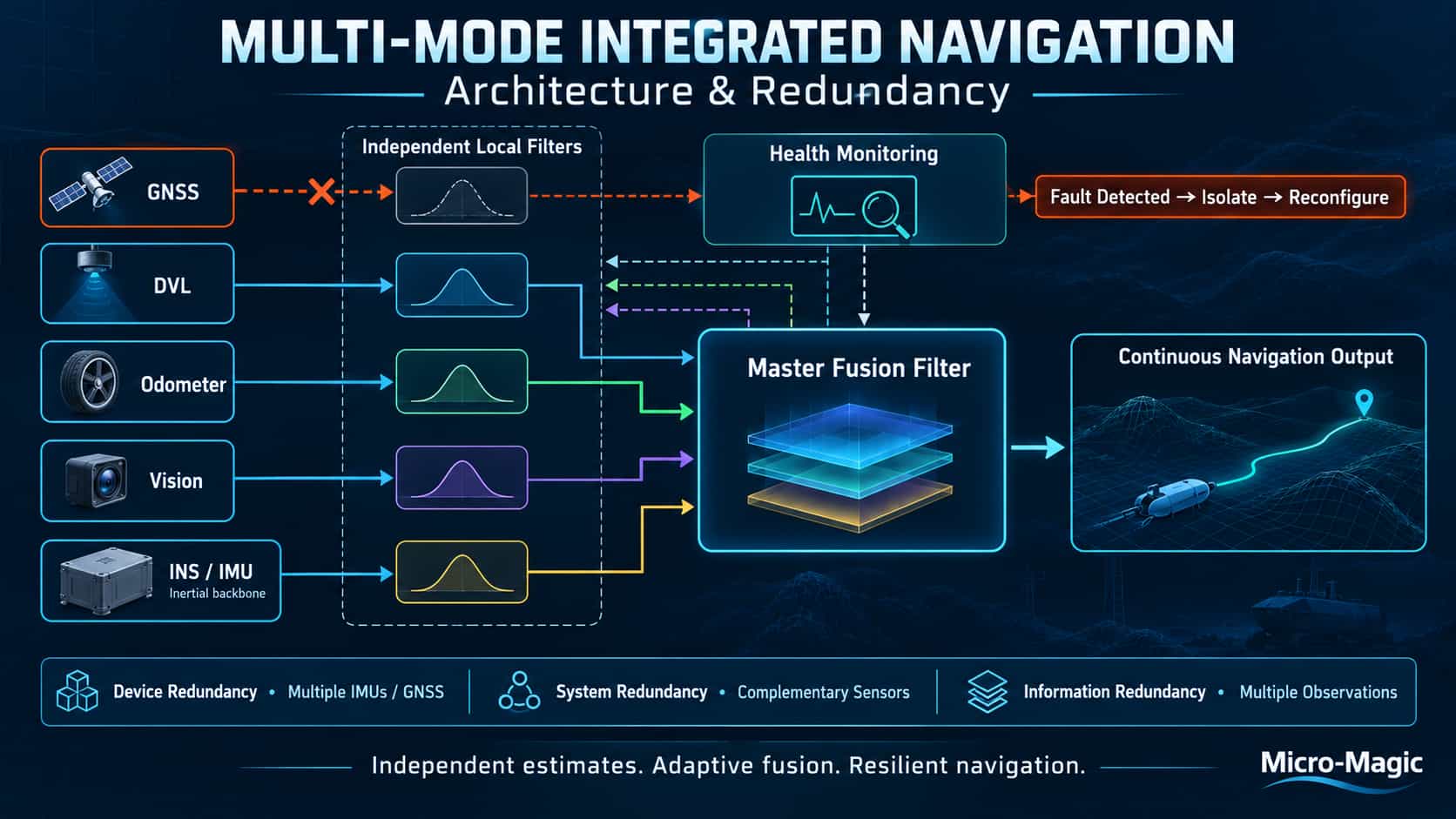
1. Introduction: From Single Sensors to Multi-Source Fusion A single navigation sensor cannot simultaneously meet requirements for accuracy, reliability, and continuity across all operating conditions. While Inertial Navigation Systems (INS) offer the advantages of full autonomy and high output rates, their errors grow without bound over time; conversely, Global Navigation Satellite Systems (GNSS) provide a stable, long-term absolute position reference but are susceptible to signal blockage and interference. This gives rise to the core concept of integrated navigation systems: using a computer as the central hub to synthesize and mathematically optimize data from multiple navigation sensors, thereby achieving "complementary strengths and synergistic performance." Building on this, redundant design addresses a critical issue in functional safety—ensuring the system maintains normal navigation capabilities even when a specific sensor malfunctions. 2. Overall Architecture: The Federated Filtering Framework Modern multi-mode integrated navigation systems commonly employ the Federated Kalman Filter architecture. Positioned between centralized and fully decentralized filtering, this structure strikes a balance between optimality and fault tolerance. 最小化图片 编辑图片 删除图片 Structural Composition The basic structure of a federated filter consists of a master filter and N sub-filters. Each sub-filter independently processes observation data from a sensor subsystem, while the master filter is responsible for the globally optimal fusion of the local estimates from the sub-filters. Core Fusion Formula: Let $\hat{X}_i$ be the state estimate and $P_{ii}$ be the estimation error covariance of the $i$-th sub-filter. If the local estimates are mutually uncorrelated, the globally optimal estimate is: 最小化图片 编辑图片 删除图片 The meaning of this formula is intuitive: sub-filters with lower estimation accuracy (indicated by a larger $P_{ii}$) are assigned lower weights in the global fusion process, thereby achieving dynamic weighting based on the principle of "trusting the most accurate." Information Allocation Principle The federated filter distributes the total system information among the sub-filters and the master filter using information allocation coefficients Bi 最小化图片 编辑图片 删除图片 Here, Q represents the system process noise covariance matrix. The information allocation strategy determines the trade-off between system accuracy and fault tolerance. A comparison of four typical operating modes is presented below: Due to the mutual isolation of the sub-filters in the NR mode, faults do not cause cross-contamination; consequently, it offers the highest fault tolerance and is best suited for fault detection and isolation. 3. Redundancy Design Concepts: From Component Redundancy to System Redundancy 3.1. Levels of Redundancy The redundancy design of integrated navigation systems can be categorized into three levels: (1) Component-level redundancy: Configuring multiple IMUs or multi-antenna GNSS receivers. Multi-IMU redundancy mitigates the impact of inertial drift; experiments show that a federated filtering architecture combined with multi-IMU redundancy maintains a positioning accuracy of approximately 1 meter during total GNSS failure, reducing errors by over 40% compared to single-IMU solutions. (2) System-level redundancy: Integrating heterogeneous sensors (e.g., INS, GNSS, odometer, and vision) to form a triple or multi-redundant navigation architecture. When GNSS signals fail—such as in tunnels or urban canyons—odometry and vision complement the INS, ensuring continuous, high-precision navigation output. (3) Information redundancy: A single sensor provides multiple types of observation data. For instance, GNSS can simultaneously output pseudorange, pseudorange rate, and carrier phase; raw multi-beam data from an LDV (Laser Doppler Velocimeter) can serve as redundant observations directly within a tightly coupled filtering framework. 3.2. Fault Detection and Isolation Mechanisms The value of redundancy design lies in the system's ability to respond to faults. Typical mechanisms include: Cross-voting: Voting among multiple redundant solution outputs to select the most consistent result and isolate anomalous observations that deviate significantly. Residual Chi-square test: Monitoring the statistical properties of the filter innovation (residual) to determine if observations are anomalous. LOF (Local Outlier Factor) detection: More sensitive to nonlinear scenarios and complex outliers; it can also detect violations of dynamic constraints (such as the zero-sideslip assumption). 3.3. Case Study: Redundancy Combinations in Engineering Practice A typical redundancy architecture for vehicle-based integrated navigation systems can be summarized as a GNSS/INS/OD (Odometer) triple-redundancy configuration. By deeply integrating vehicle odometer data, the system maintains continuous, high-precision navigation output even in GNSS-denied environments and enables seamless switching between various operating modes. Conclusion The overall architecture of the multi-mode integrated navigation system utilizes federated filtering as the core fusion mechanism and redundant design to ensure reliability. The systems engineering philosophy underpinning this combination can be summarized as follows: independent optimal estimation by individual sensors, globally optimal fusion via a master filter, and rapid fault isolation and system reconfiguration. This architecture achieves a balance among accuracy, reliability, and environmental adaptability, serving as a core technological foundation for fields such as autonomous driving, unmanned aerial vehicles (UAVs), and marine navigation.

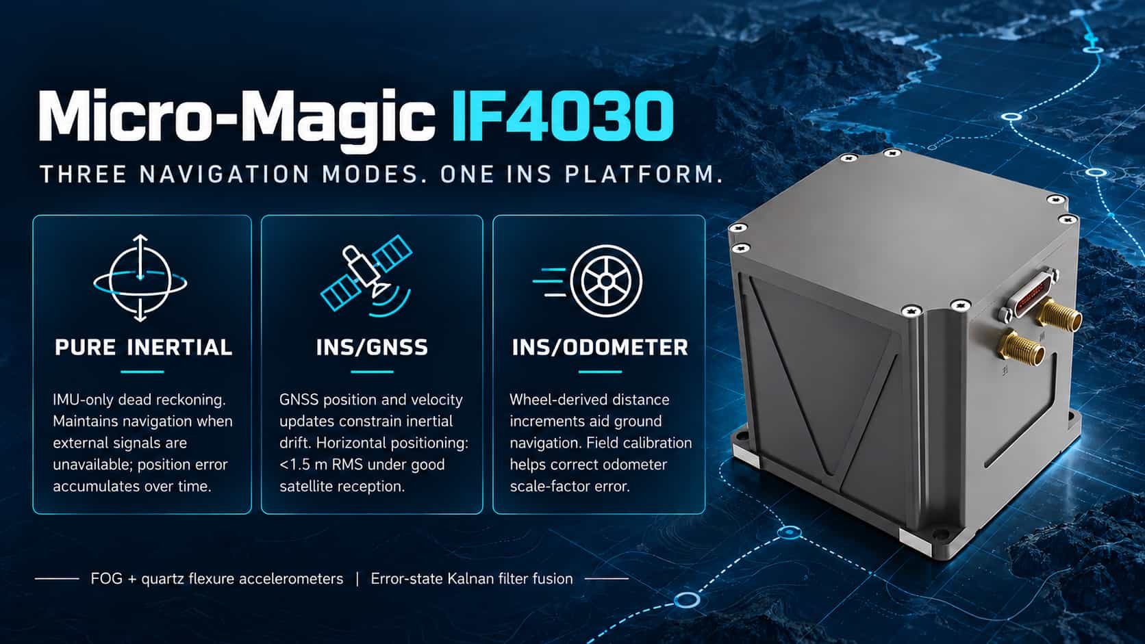
The IF4030 fiber-optic inertial navigation system supports six standardized operating modes, covering typical mission scenarios across land, sea, air, and underwater domains; flexible adaptation is achieved through sensor fusion and algorithmic switching. Pure Inertial Mode Relies entirely on internal gyroscopes and accelerometers for dead reckoning, without external data. Following power-on self-test and a 275-second static alignment, the system enters pure inertial navigation mode, achieving a heading accuracy of 0.1–0.2°/h and a position accuracy of 2.5–6 nmi/h (CEP). Suitable for contingency scenarios such as GNSS-denied environments, tunnels, or areas with strong electromagnetic interference. Inertial/Satellite Integrated Mode Utilizes tight coupling with GNSS (GPS/BDS/GLONASS) observations. When satellite signals are available, horizontal positioning accuracy exceeds 1.5 m and vertical accuracy exceeds 3 m (single-point positioning), with a velocity accuracy of 0.02 m/s (RMS). It supports RTK differential positioning for centimeter-level accuracy and satellite-aided moving-base alignment (approx. 15 minutes). The system maintains continuous output during brief signal outages and automatically converges upon signal re-acquisition; suitable for applications such as UAVs and electro-optical (EO) pods. Inertial/DVL Integrated Mode Integrates velocity data (bottom-track or water-track) from a Doppler Velocity Log (DVL) to effectively suppress velocity drift inherent in pure inertial systems; designed for underwater robots (ROV/AUV) and marine platforms. Supports axis configuration and lever-arm compensation, automatically identifying BS/BI data for velocity matching. Inertial/Odometer Integrated Mode Designed for ground vehicles and track inspection vehicles; integrates pulse signals from wheel odometers to maintain sub-meter/kilometer positioning accuracy in long tunnels or mining areas where satellite signals are unavailable. Supports online scale factor calibration and installation misalignment correction, with automatic storage of calibration parameters via route-based calibration. Inertial/Visual Fusion Mode This mode receives visual odometry or SLAM pose data via Ethernet or serial port; visual data constrains inertial drift, while inertial data smooths out visual noise. It is suitable for UAVs or service robots operating in GNSS-denied indoor environments and requires factory-level joint calibration. Compass (Marine Compass) Mode In this mode, once the inertial navigation system enters the navigation state, it continuously outputs a highly stable heading using purely inertial methods. The core principle involves using a gyro-compassing algorithm to sense the Earth's rotational angular velocity vector and determine True North. It is suitable for surface vessels and operations in polar or high-latitude regions. The system allows users to select the primary fusion scenario (land, marine, or aerial) and configure output priorities via parameter settings. It automatically degrades performance if an auxiliary sensor fails, ensuring continuous and reliable navigation. Real-time mode switching and status monitoring are supported to accommodate diverse mission planning requirements.

1. Overview The IF4030 series fiber-optic inertial navigation systems are engineered according to SWaP (Size, Weight, and Power) optimization principles—prioritizing miniaturization, lightweight construction, and low power consumption—while maintaining high reliability and the ability to operate across a wide temperature range. Physical dimensions and interfaces are standardized across models of varying precision levels; users do not need to modify mechanical or electrical designs when selecting different precision grades, and this platform-based approach significantly reduces system integration costs. Key specifications include: dimensions of 80 × 80 × 84 mm, a weight of 0.9 kg, a supply voltage of 12–36 V, a maximum power consumption of less than 12 W, an operating temperature range of -45°C to 70°C, and electromagnetic compatibility (EMC) that meets GJB151B standards for Air Force aircraft. 2. Dimensional Analysis The IF4030 is relatively compact compared to similar fiber-optic inertial navigation systems. Through the miniaturization of optical paths and 3D stacked circuit board layouts, its volume has been reduced by approximately 40%, making it particularly suitable for space-constrained applications such as small UAV compartments, electro-optical (EO) pods, and the sealed hulls of underwater robots. The mounting surface requires a flatness better than 0.05 mm, a factor directly influencing attitude output accuracy. An azimuth mounting surface is provided on the side of the housing to ensure precise alignment with the host platform's reference plane. By default, the Y-axis points in the direction of the host platform's forward motion; incorrect installation will result in systematic navigation errors. The coordinate system follows the "Right-Forward-Up" convention, consistent with standard practices in aviation and marine inertial navigation. Its 0.9 kg mass results in a high mechanical resonant frequency, which helps suppress vibration-induced interference on inertial components and minimizes lever-arm effect errors caused by the flexural deformation of mounting brackets. 3. Weight Analysis The unit integrates three fiber-optic gyroscopes, three quartz flexure accelerometers, a power supply module, a data acquisition and processing module, and a satellite navigation module. The power-to-weight ratio is approximately 13 W/kg, performing far better than comparable products, which typically range from 25 W/kg to 40 W/kg. For multi-rotor UAVs, every 100g reduction in weight extends flight endurance by approximately two to three minutes; the 0.9 kg weight significantly frees up payload capacity. Regarding mass distribution, the fiber-optic gyroscope (FOG) assembly accounts for about 35% of the total weight, making it the heaviest component; the three precision variants share a unified platform, with differences in accuracy stemming from fiber length or coil winding techniques rather than structural changes. The aluminum alloy housing accounts for approximately 30% of the weight, balancing structural strength with heat dissipation. 4. Power Consumption Analysis Maximum power consumption is below 12 W; based on a nominal 28 V supply, the typical current draw is approximately 0.43 A. The power distribution is as follows: the FOG light source accounts for about 40% of total power consumption, the accelerometer servo consumes 0.5–1 W, the computing module 2–3 W, the satellite receiver 1–1.5 W, and power conversion losses account for 1–2 W. Power consumption below 12 W reduces heat accumulation in the sealed enclosure. The fanless, passive cooling design eliminates moving parts and enhances long-term reliability, offering particular advantages for battery-powered platforms. Regarding power protection, voltages exceeding 36 V may damage components, while voltages below 12 V trigger an undervoltage lockout (UVLO) resulting in a system reset; the system includes built-in reverse polarity protection and features transient voltage suppression (TVS) devices at the front end. 5. Operating Temperature Range Analysis The wide operating temperature range of -45°C to +70°C complies with the GJB150A military standard, making the system suitable for extreme environments such as high-latitude cold regions, high-altitude UAV operations, and high-temperature desert conditions. FOG bias is highly sensitive to temperature, with drift comprising linear, quadratic, and hysteresis components. For the high-precision model (with a bias stability of 0.06°/h), the residual error after temperature compensation is required to remain within 0.02°/h, assuming a temperature change rate of no more than 1°C per minute. The system utilizes full-temperature-range calibration to store compensation parameters in flash memory, applying real-time compensation based on temperature sensor readings during navigation. 6. Integration Considerations Compared to typical tactical-grade fiber-optic inertial navigation systems, the IF4030 offers a volume reduction of approximately 40%, a weight reduction of over 50%, and a power consumption reduction of about 40%; it operates over a wider temperature range while delivering equivalent accuracy. Key integration requirements include: ensuring the flatness of the mounting surface, as stress-induced deformation can affect the fiber-optic coil's bias stability; limiting the power input to the 12V–36V range and configuring front-end protection and filtering; and ensuring effective thermal conduction between the mounting surface and the structure in high-temperature environments. The standardized form factor allows users to upgrade accuracy without redesigning mounting or power supply configurations.

System Positioning and Accuracy Class The IF4030 series comprises high-performance Inertial Navigation Systems (INS) based on fiber-optic gyroscopes (FOG) and quartz flexure accelerometers. Designed to balance miniaturization (80mm × 80mm × 84mm, 0.9kg) with high precision, the series targets platforms such as medium-sized UAVs, optoelectronic pods, and underwater robots—applications that are sensitive to SWaP (Size, Weight, and Power) constraints yet require moderate-to-high navigation accuracy. The series is categorized into three models based on north-finding accuracy: 最小化图片 编辑图片 删除图片 Here, φ represents the local latitude; the fact that the north-finding error increases with latitude is determined by the attenuation of the horizontal component of the Earth's angular velocity (Ω·cosφ) as latitude rises. Since north-finding accuracy is inversely proportional to cosφ, longer integration times or higher-precision gyroscopes are required to compensate in high-latitude regions. Core Parameter Framework and Error Models (1) Inertial Component Specifications 最小化图片 编辑图片 删除图片