
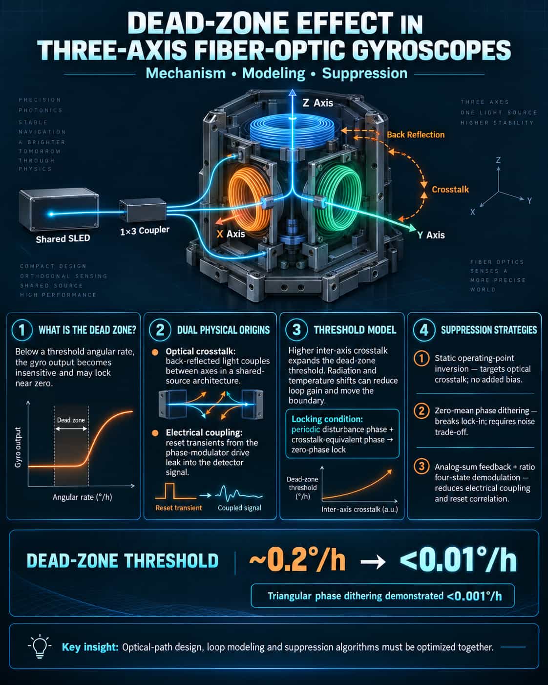
As three-axis fiber-optic gyroscopes (FOGs) increasingly aim for miniaturization and high precision, the "dead-zone" effect—triggered by inter-axis optical crosstalk—has become a critical bottleneck limiting performance in low-angular-rate measurements. A dead zone occurs when the gyroscope's output ceases to respond to changes in input angular velocity below a certain threshold. For applications such as satellite attitude control that require operation near zero angular velocity, the nonlinear bias error introduced by the dead zone directly compromises system accuracy. This paper focuses on the issue of inter-axis optical crosstalk in three-axis FOGs utilizing a shared-light-source architecture; it analyzes the underlying physical mechanisms, quantifies the impact on threshold characteristics, and comparatively evaluates current primary mitigation strategies. **Physical Origins of the Dead Zone and the Inter-Axis Optical Crosstalk Model** The dead zone is a nonlinear effect characteristic of digital closed-loop FOGs. Conventionally, the primary source of interference causing the dead zone is identified as the electrical cross-coupling of the staircase voltage applied to the phase modulator into the detector signal. However, in a three-axis shared-source architecture, the problem is more complex: a single superluminescent diode (SLD) source drives three orthogonal axes simultaneously after being split by a 1×3 coupler. Back-reflected light creates optical crosstalk channels between the axes; at low angular rates, this optical intensity crosstalk superimposes onto the interference intensity, potentially overwhelming the useful signal. To quantitatively characterize this effect, a study proposed an open-loop excitation method to measure the optical back-reflection crosstalk coefficients between axes. Incorporating these coefficients into a closed-loop control model reveals that an increase in the crosstalk coefficient causes the gyroscope's threshold to expand multiplicatively, directly resulting in a wider dead-zone range. This mechanism can be formalized as follows: when the phase of the periodic disturbance in the feedback channel and the equivalent phase of the crosstalk satisfy specific conditions, the system enters the dead zone, and the output phase locks to zero. **Quantitative Characterization of Dead-Zone Thresholds** The impact of the dead zone on the system lies not only in the existence of an "insensitive range" but also in the fact that the boundaries of this range shift dynamically due to environmental factors such as space radiation and temperature fluctuations. Space radiation causes a decrease in light source power and an increase in fiber loss, thereby reducing the system gain (K₁) and expanding the dead-zone range. Experimental data indicate that the dead-zone threshold of an uncompensated triaxial gyroscope can reach the order of 0.2°/h, a level unacceptable for high-precision applications requiring the resolution of extremely low angular velocities. It is worth noting that the dead zone arises from multiple mechanisms. In addition to inter-axis optical crosstalk, electrical cross-coupling constitutes another significant cause. The analog drive voltage signal of the phase modulator—subjected to resets via a digital feedback staircase wave—generates distinct operating modes; the resulting crosstalk, manifesting as variations in the amplitude and phase of the detector output signal, becomes particularly pronounced during state transitions in the four-state modulation scheme. Since these two mechanisms often act concurrently in triaxial systems, modeling the dead zone requires accounting for both optical and electrical dimensions. Comparative Analysis of Suppression Schemes To address the aforementioned causes of dead zones, three primary suppression strategies have been developed, each differing in mechanism and effectiveness: Static operating point flipping (bias switching) method. Targeting the physical root cause of inter-axis optical crosstalk, this method actively flips the gyroscope's static operating point so that the crosstalk signal no longer superimposes onto the closed-loop residual phase. Experimental results are impressive: this approach reduces the threshold from 0.2°/h to below 0.01°/h, effectively enhancing measurement accuracy at low rotation rates. Its advantage lies in directly addressing the optical crosstalk mechanism without introducing additional bias errors. Periodic perturbation superposition method (dithering). A zero-mean periodic perturbation phase, φ₀, is introduced into the system to break the dead-zone locking condition through "dithering." When the dither amplitude is sufficiently large (φ₀ ≥ φ₁), the dead zone can be completely eliminated. In practical engineering applications, triangular-wave phase dithering technology has suppressed the dead-zone error of high-precision gyroscopes from 0.08°/h to below 0.001°/h. The method's effectiveness has been validated in a triaxial system utilizing 900 meters of optical fiber; suppression performance depends on the specific combination of dither amplitude, frequency, and loop gain. However, excessive dither amplitude may introduce additional noise, necessitating a careful trade-off. Combined method of analog additive feedback and ratio-based four-state demodulation. This method addresses the issue starting with the electrical cross-coupling path: in traditional four-state modulation, the reset operations associated with each modulation state are a primary cause of the dead zone. The analog additive feedback method significantly reduces the frequency of reset operations by resetting only the feedback phase during modulation; experiments demonstrate that this can lower the dead zone to below the measurement threshold of 0.022°/h. However, due to the inherent nature of electrical crosstalk, this method still introduces an additional bias of approximately -0.06°/h. To mitigate this, the method is further combined with the ratio-based four-state demodulation technique; by adjusting the demodulation ratio of the feedback signal, the correlation between the modulation and demodulation sequences is weakened, thereby controlling the additional bias while simultaneously suppressing the dead zone. Overall, these three types of schemes are suited to different application scenarios: the optical crosstalk suppression scheme is most effective for tri-axial architectures sharing a common light source; the dithering method is simple to implement but requires noise management; and electrical crosstalk suppression schemes are better suited for single-axis and discrete systems. For silicon-photonic gyroscopes aiming for ultra-high integration, recent research has introduced a joint suppression algorithm that integrates phase-shift hopping with sample rejection; this approach suppresses the dead zone while reducing angle random walk by over 26%, reflecting a trend toward combining multiple strategies rather than relying on a single method. In summary, the dead zone effect in tri-axial fiber-optic gyroscopes is a systemic issue resulting from the coupling of multiple factors. Inter-axis optical crosstalk and electrical cross-coupling constitute the physical root causes of the dead zone, with their effects significantly amplified in architectures featuring common light sources and high levels of integration. Currently, the static operating point bias-flipping method offers the best performance for optical crosstalk suppression, the dithering method boasts the broadest applicability, and combined modulation schemes represent the cutting edge of electrical crosstalk suppression. As tri-axial gyroscopes evolve toward chip-scale integration, the combination of inter-waveguide crosstalk suppression (e.g., germanium-doped silica waveguide chips achieving crosstalk levels below -40 dB) and algorithmic joint suppression strategies may well become the key pathway to completely resolving the dead zone problem.
Read More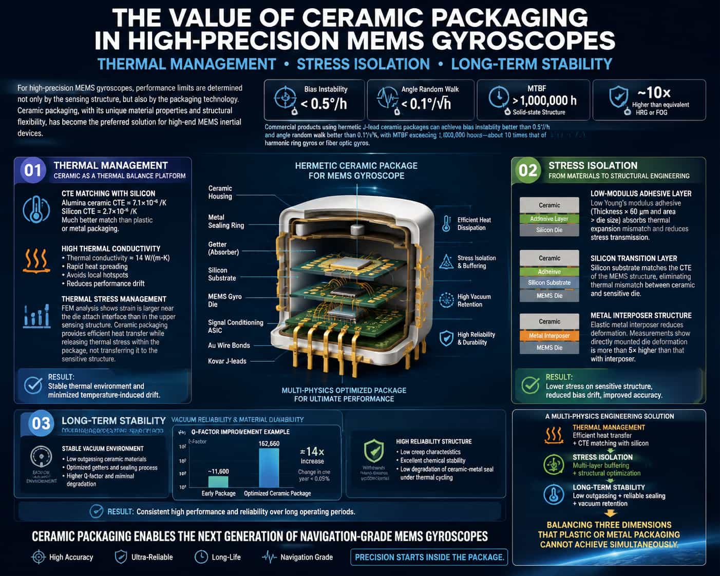
The performance limits of high-precision MEMS gyroscopes are largely determined by their packaging solutions rather than solely by the design of the sensing structure. Thanks to their unique material properties and structural flexibility, ceramic packages have become the preferred choice for high-end MEMS inertial devices. Currently, commercial high-performance MEMS gyroscopes utilizing hermetic J-lead ceramic packages achieve bias stability better than 0.5°/h and angular random walk better than 0.1°/√h. Their solid-state structure yields a mean time between failures (MTBF) exceeding one million hours—up to ten times that of dynamically tuned gyroscopes or fiber-optic gyroscopes with comparable performance. This level of performance is underpinned by the deep optimization of ceramic packaging across three dimensions: thermal management, stress isolation, and long-term stability. Thermal Management: Ceramics as a Thermal Equilibrium Platform The value of ceramic packaging in thermal management is primarily demonstrated by the favorable match between its coefficient of thermal expansion (CTE) and that of silicon. While the CTE of alumina ceramic (approx. 7.1 × 10⁻⁶/K) differs from that of silicon (2.7 × 10⁻⁶/K), the match is significantly better than that offered by plastic or metal packaging. More importantly, the high thermal conductivity of ceramics (approx. 14 W/(m·K)) allows for the rapid dissipation of heat generated by the sensing structure into the external environment, preventing performance drift caused by localized hot spots. Finite element analysis reveals a distinct gradient distribution of stress and strain within the MEMS gyroscope chip: strain in the upper sensing structure is lower than that near the lower bonding interface, and strain in the rigid support pillars and chip edges is lower than in the cavity structure regions. This pattern highlights a critical conflict in thermal management: while packaging materials require high thermal conductivity to achieve thermal equilibrium, the heat conduction path itself can serve as a channel for stress transmission. Ceramic packaging addresses this by facilitating efficient heat conduction while employing structural designs that allow thermal stress to be partially relieved at the package level, rather than being transmitted directly to the sensing structure. Stress Isolation: From Material Selection to Structural Engineering Thermal stress within the package is the primary factor limiting the performance of MEMS gyroscopes. Simulation and experimental studies indicate that the degree of matching between the coefficients of thermal expansion (CTEs) of the ceramic substrate/adhesive and the silicon, as well as the Young's modulus of the adhesive, directly influence the level of thermal stress within the package. Thermal stress can be effectively controlled when the adhesive has a low Young's modulus, the adhesive layer exceeds 60 μm in thickness, and its planar dimensions are larger than those of the chip. The underlying physical mechanism is that the low-modulus adhesive layer acts as a buffer medium; it absorbs the strain energy resulting from thermal expansion mismatch through its own deformation, thereby reducing the stress transmitted to the sensitive structures. More advanced stress isolation strategies involve multi-layer structural designs. The 214th Institute of China North Industries Group Corporation (NORINCO) proposed a low-stress packaging scheme: a silicon substrate is bonded to the bottom of a ceramic package housing, with both the MEMS sensitive structure and signal processing circuitry bonded onto the silicon substrate and electrically connected via gold wire bonding. Serving as a transition layer, the silicon substrate possesses a CTE identical to that of the sensitive structure, thereby eliminating the thermal mismatch issues that would arise from direct contact between the sensitive structure and the ceramic substrate. Building upon this, the use of a localized five-point bonding method—combined with the incorporation of small-diameter glass beads into the adhesive to act as a buffer—can further mitigate thermal stress effects and enhance resistance to high-G loads. International research has also validated similar approaches. By installing an elastic metal interposer within the ceramic chip carrier, the temperature drift of the scale factor and bias in tuning-fork gyroscopes has been significantly suppressed. Holographic interferometry has confirmed that the deformation of a sensitive chip directly brazed to the package is more than five times greater than that of a chip mounted via an interposer. This interposer structure is fabricated from chemically etched metal foil; following gold plating, it is bonded to both the sensor chip and the ceramic package using thermocompression bonding, achieving stress isolation while maintaining mechanical connection stability. Long-term Stability: Vacuum Maintenance and Material Outgassing Control The contribution of ceramic packaging to long-term stability lies primarily in its ability to maintain a vacuum environment over an extended period. The quality factor (Q-value) of a MEMS gyroscope is closely linked to gas damping within the cavity; a decline in the Q-value directly leads to the degradation of bias stability and scale factor stability. Research indicates that the primary cause of Q-value degradation in early vacuum-packaged gyroscopes was the continuous outgassing of residual gases within the cavity. By analyzing the outgassing characteristics of ceramic packages and metal lids using Temperature-Programmed Desorption Mass Spectrometry (TPD-MS)—and subsequently selecting appropriate getters and refining the packaging process—the gyroscope's Q-factor was increased to 162,660. This represents a roughly fourteen-fold improvement over earlier packaging iterations, with a variation of less than 0.05% over the course of a year. These data demonstrate that the long-term stability of the gyroscope is collectively determined by the outgassing rate of the ceramic material itself, the long-term hermeticity of the sealing interface, and the effectiveness of the internal getter. Another advantage of ceramic packaging regarding long-term stability lies in its fatigue resistance. Compared to plastic or metal packaging, ceramic-to-metal sealing interfaces exhibit a slower rate of degradation under thermal cycling conditions. The use of ceramic packaging in the GYPRO4300 enables it to meet the rigorous thermal cycling requirements of critical applications, maintaining high reliability even under harsh conditions involving rapid temperature fluctuations—a testament to the low creep and chemical inertness of ceramic materials. In summary, the value of ceramic packaging for high-precision MEMS gyroscopes cannot be reduced merely to "material selection." It represents a system-level engineering challenge involving multi-physics coupling: thermal management requires the ceramic substrate to possess good thermal conductivity and a Coefficient of Thermal Expansion (CTE) matched to silicon; stress isolation necessitates multi-stage buffer structures, such as low-modulus adhesive layers, silicon interposers, or metal intermediate layers; and long-term stability relies on the comprehensive optimization of ceramic low-outgassing properties, seal durability, and vacuum retention technology. The success of the ceramic packaging solution lies precisely in its ability to strike a balance across these three dimensions—a feat often difficult to achieve simultaneously with plastic or metal packaging. As MEMS gyroscopes advance toward navigation-grade precision, technological innovation at the packaging level will remain a critical pathway for overcoming performance bottlenecks.
Read More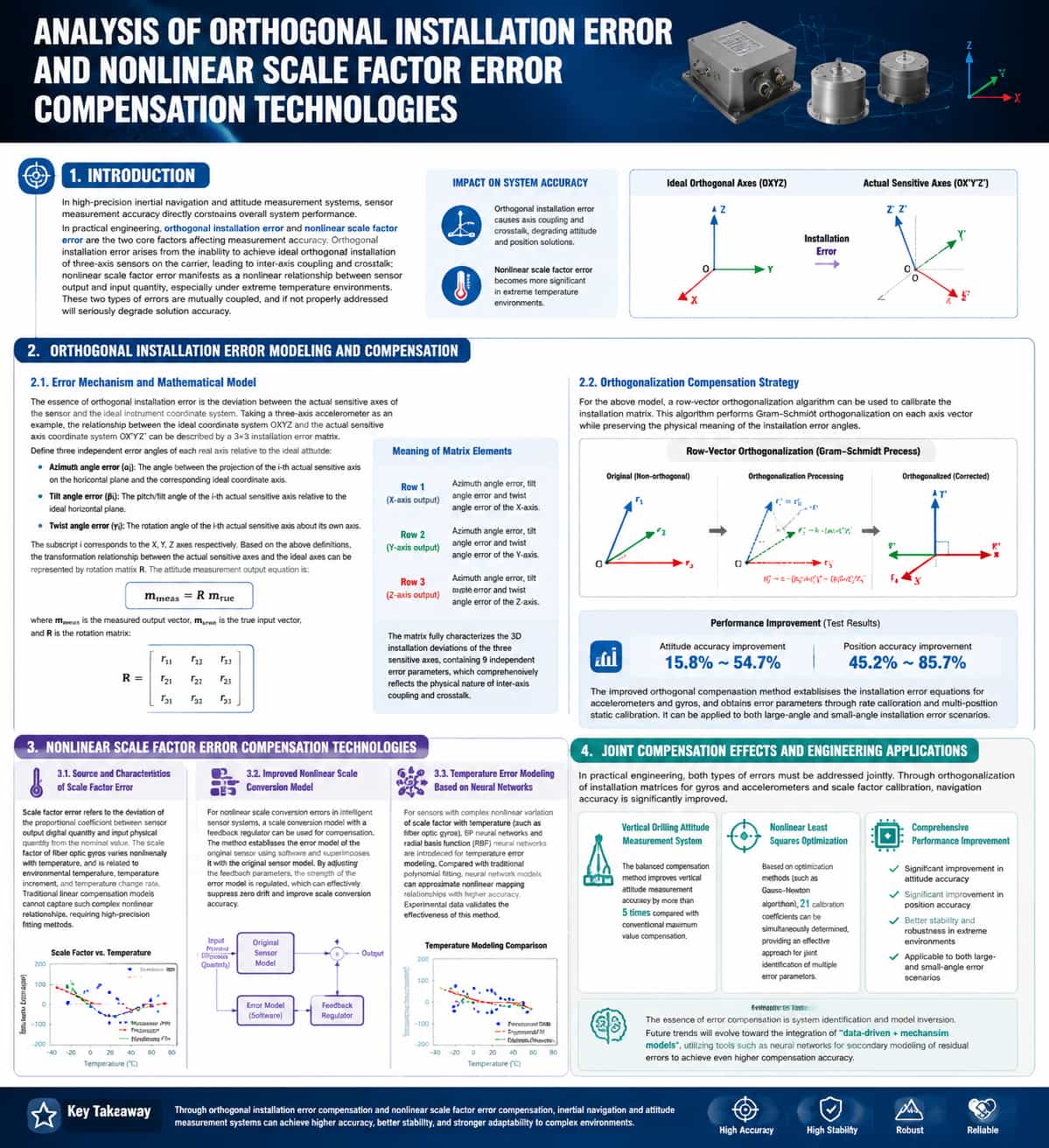
Introduction In high-precision inertial navigation and attitude measurement systems, sensor measurement accuracy directly constrains the system's overall performance. In practical engineering applications, non-orthogonal mounting errors and nonlinear scale errors are the two primary factors affecting measurement accuracy. Non-orthogonal mounting errors arise from the inability to achieve ideal orthogonal mounting of the tri-axial sensors on the carrier, resulting in inter-axis coupling and crosstalk; nonlinear scale errors manifest as a nonlinear relationship between sensor output and input, a phenomenon particularly pronounced in extreme temperature environments. These two types of errors are coupled; if not properly addressed, they can severely degrade the accuracy of the navigation solution. Modeling and Compensation of Non-orthogonal Mounting Errors Error Mechanism and Mathematical Model The essence of non-orthogonal mounting error lies in the deviation between the sensor's actual sensitive axes and the ideal instrument coordinate system. Taking a tri-axial accelerometer as an example, let OXYZ denote the ideal coordinate system and OX′Y′Z′ denote the coordinate system of the actual sensitive axes; the relationship between them can be described by a 3×3 mounting error matrix. To precisely characterize this error, three independent error angles for each actual axis relative to the ideal orientation are defined as follows: (Azimuth error): The angle between the projection of the i-th actual sensitive axis onto the horizontal plane and the direction of the ideal coordinate axis. (Tilt error): The pitch/tilt angle of the i-th actual sensitive axis relative to the ideal horizontal plane. (Torsion error): The rotation angle of the i-th actual sensitive axis about its own axis. Here, the subscript corresponds to the X, Y, and Z axes, respectively. Based on these definitions, the transformation relationship between the actual sensitive axes and the ideal axes can be represented by a rotation matrix R, and the attitude measurement output equation is: The rotation matrix R is: The specific meanings of the elements in the matrix are described as follows: Row 1 (corresponding to the actual X-axis output): represent the azimuth angle error, tilt angle error, and torsion angle error of the X-axis, respectively. Row 2 (corresponding to the actual Y-axis output): represent the azimuth angle error, tilt angle error, and torsion angle error of the Y-axis, respectively. Row 3 (corresponding to the actual Z-axis output):
Read More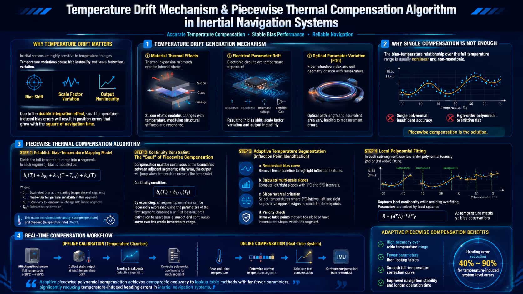
The core components of Inertial Navigation Systems (INS)—gyroscopes and accelerometers—are extremely sensitive to temperature fluctuations. This sensitivity stems from the temperature dependence of material physical properties: variations in the elastic modulus of silicon microstructures; thermal stresses caused by the mismatch in coefficients of thermal expansion (CTE) between silicon and glass in MEMS packaging; changes in optical fiber refractive index and coil geometry in fiber-optic gyroscopes; and temperature-induced drift in reference voltages and amplifier gains within electronic circuits. Temperature drift is particularly critical due to the "double-integration amplification effect": a temperature-induced bias shift, when subjected to the double integration inherent in navigation calculations, results in a positioning error that diverges quadratically with navigation time. Research indicates that the temperature drift coefficient for MEMS accelerometers can reach 0.54 mg/°C, while the bias instability of MEMS gyroscopes over a wide temperature range can reach 4.6°/h—levels that are unacceptable for tactical-grade applications. Drift mechanisms can be categorized into three types: · Thermal effects on materials: CTE mismatch between silicon and packaging materials generates thermal stress, altering the stiffness and resonant frequency of the sensing structure. · Electrical parameter drift: Temperature-induced changes in resistors, capacitors, and reference voltages within the detection circuitry alter the sensor's scale factor and zero-offset. · Optical parameter variations (fiber-optic gyroscopes): Changes in the optical fiber's refractive index, combined with the thermal expansion and contraction of the fiber coil, alter the optical path length and equivalent area. Mathematical Principles of Piecewise Temperature Drift Compensation Algorithms The core task of temperature drift compensation is to establish a mapping model between bias and temperature—that is, to solve for the error function: Here, "bias" represents the zero-offset of the gyroscope or accelerometer, and T denotes temperature. In engineering practice, the function f(T) across the full temperature range often exhibits nonlinear or even non-monotonic characteristics; fitting this range with a single polynomial results in either insufficient accuracy or overfitting due to an excessively high polynomial order. Consequently, the piecewise compensation strategy was developed. Basic form of the piecewise model Divide the entire temperature range into n temperature intervals ; within the j-th interval, the bias is expressed as a function of temperature and its rate of change: Where: is the equivalent bias at the starting temperature point of segment $j$; is the first-order sensitivity coefficient of the bias to temperature within that segment; is the sensitivity coefficient of the bias to the rate of temperature change within that segment; is the reference temperature. This model accounts for both steady-state temperature effects (the second term) and dynamic temperature effects (the third term)—the latter being particularly critical during the warm-up phase following startup. (2) Continuity constraint: the "soul" of piecewise compensation A critical constraint for piecewise compensation is that the compensation values must be continuous at the boundaries between adjacent temperature segments; otherwise, a sudden jump in the output would occur as the temperature slowly crosses the inflection point, leading to discontinuity in the navigation solution. The continuity condition can be expressed as: Upon expansion, the bias of each segment can be expressed recursively in terms of the parameters of the first segment; this allows the fitting parameters for all segments to be treated as a unified whole for least-squares estimation, thereby ensuring the smoothness and continuity of the curve across the entire temperature range. (3) Inflection Point Identification and Adaptive Segmentation Segmentation hinges on identifying inflection points—temperature nodes where the slope of the temperature-bias curve changes significantly. An adaptive inflection point identification algorithm is employed in engineering practice, with the following core logic: a. Reconstruct the bias curve: Subtract the linear baseline (calculated over the full temperature range) from the raw bias data to accentuate the characteristics of the inflection points. b. Calculate multi-scale slopes: Compute the left and right slopes at intervals of 1°C and 5°C, respectively. c. Slope sign criterion: Identify temperature points where the signs of the left and right slopes (at the 5°C interval) differ; designate these as candidate inflection points. d. Validity check: Eliminate "pseudo-inflection points" that are spaced too closely or lack sufficient slope consistency within the interval. Once inflection points are identified, low-order polynomial fitting (typically second or third-order) is applied within each sub-interval; this approach captures local nonlinearity while avoiding overfitting. The fitting parameters are determined using the least-squares method: Here, Temp is the temperature matrix, and B represents the corresponding bias observations. Real-time compensation process In actual engineering implementation, segmented temperature drift compensation is divided into two stages: · Offline calibration stage: The IMU is placed in a thermostat to perform temperature cycles across the full temperature range (such as -30°C to 70°C), record the static output at each temperature point, and complete inflection point identification and calculation of fitting parameters for each segment. · Online compensation stage: The system reads the temperature sensor value in real time, determines the range to which the current temperature belongs, substitutes it into the corresponding model to calculate the compensation amount, and deducts it from the original output: Research indicates that the adaptive piecewise polynomial method can achieve compensation accuracy comparable to that of the look-up table method while requiring significantly fewer compensation parameters. Regarding system-level heading effect errors caused by temperature fluctuations, a compensation method based on the Fourier expansion of temperature variations can reduce the error by 40% to 90%.
Read More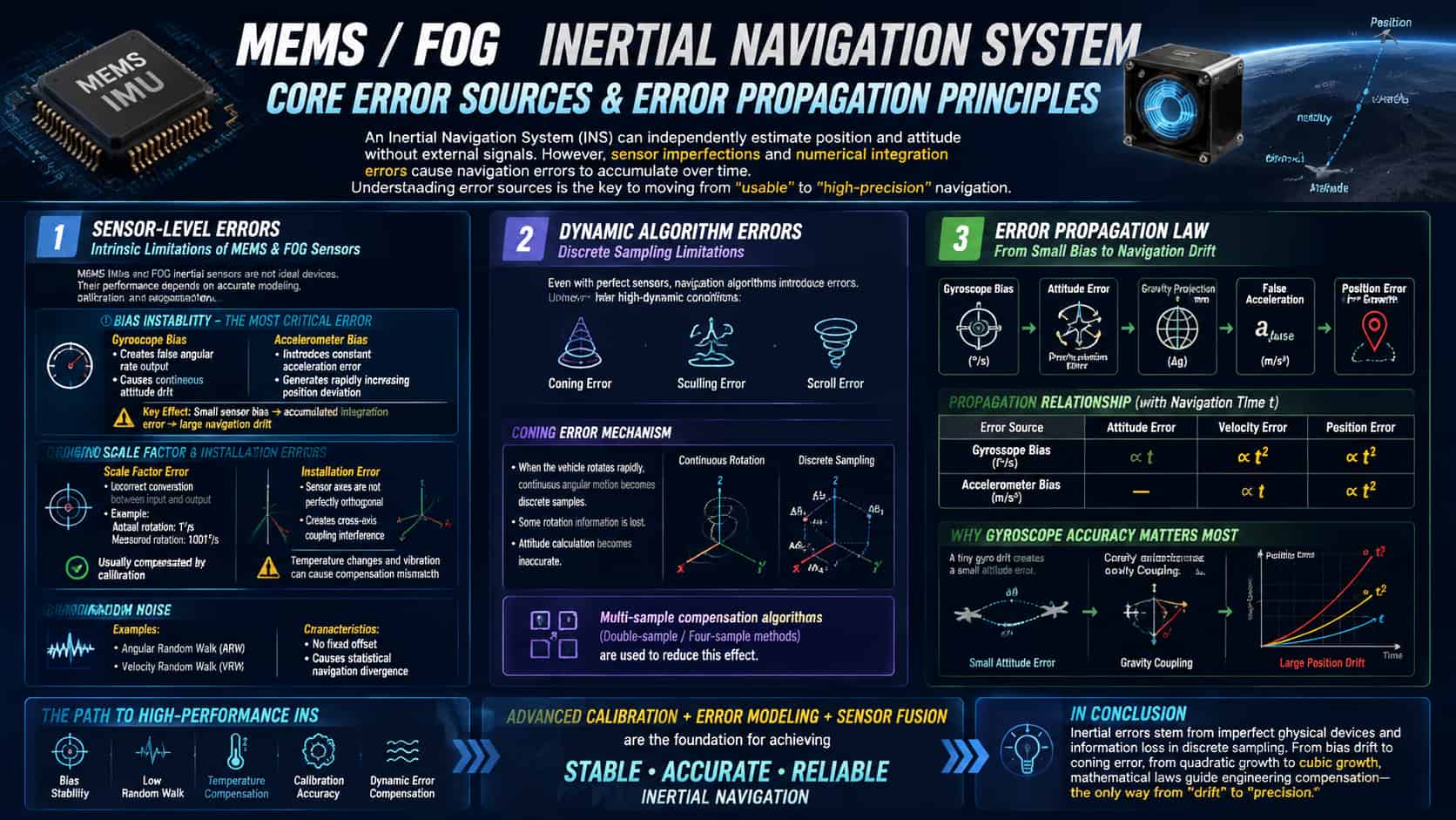
The allure of inertial navigation systems lies in their ability to autonomously calculate position and orientation without relying on any external signals. The trade-off, however, is that errors accumulate relentlessly over time. Understanding the primary sources of these errors is a crucial step in transitioning from a system that merely "works" to one that performs exceptionally well. 1. Sensor-Level Errors: The "Inherent Flaws" of the Hardware The core components of an inertial navigation system (INS)—gyroscopes and accelerometers—are not ideal sensors. Error analysis begins with modeling and quantifying these "inherent flaws." Bias is one of the most critical sources of error. A gyroscope's output of a false angular rate while stationary leads to continuous orientation drift, while an accelerometer's bias introduces a constant offset directly into specific force measurements. An accelerometer bias of just 0.1 mg can result in a positional error of approximately 50 meters within 100 seconds. The danger of bias lies not only in the offset itself but in its amplification through double integration: positional error grows in proportion to the square of time. Scale factor errors and installation errors are classified as structural errors. An inaccurate scale factor means, for instance, misinterpreting a rotation of 1°/s as 1.001°/s; installation errors result in the three sensitive axes not being perfectly orthogonal, creating cross-coupling interference. While such errors can usually be compensated for via factory calibration, temperature fluctuations and mechanical shocks can cause the compensation parameters to become mismatched. From a dynamic perspective, the angular motion of the mounting base introduces additional error terms in the gyroscope and accelerometer outputs—coupled with angular velocity and angular acceleration—that are significant enough to warrant attention. Random noise (such as angle random walk and velocity random walk), while not producing a constant offset, causes navigation errors to exhibit characteristics of statistical, random divergence. 2. Algorithm-Level Dynamic Errors: The Pitfalls of Discrete Sampling Even with perfect sensors, the numerical integration process itself introduces errors. In high-dynamic environments—characterized by factors such as high-frequency vibration and violent maneuvers—classic errors known as "coning error," "sculling error," and "scrolling error" arise. Take coning error as an example: when the angular velocity vector of the vehicle rotates rapidly in space, discrete sampling captures angular increments only at specific, finite moments. Consequently, the continuous trajectory of the rotation vector cannot be precisely reconstructed, resulting in a loss of rotational information. Multi-sample coning compensation algorithms (such as two-sample or four-sample schemes) are specifically designed to mitigate this loss of information. 3. Error Propagation: The Mathematical Progression from "Differential" to "Divergence" The fundamental error propagation characteristics of inertial navigation systems can be summarized as follows: attitude errors caused by gyroscope bias grow linearly with navigation time, velocity errors grow quadratically, and position errors grow cubically; meanwhile, velocity errors caused by accelerometer bias grow linearly with navigation time, and position errors grow quadratically. Starting from basic kinematic relationships: ideally, position is determined by the double integration of specific force: Considering a constant accelerometer bias δα (where the measured value is f̃ = f + δα), the position calculation error δr(t) is: This relationship reveals the most critical characteristic of inertial navigation errors: quadratic divergence. To illustrate with a concrete numerical example: an accelerometer bias of just 0.01 m/s² (approximately one-thousandth of the acceleration due to gravity) can result in a position error of about 50 meters within 100 seconds. The impact of gyroscope bias is even more profound. Let ε (rad/s) be the constant drift rate of the gyroscope; this directly causes the attitude error δϕ to grow linearly over time: A ttitude error causes a deviation in the gravity vector during calculation, introducing spurious acceleration; after double integration, the resulting position error is ultimately proportional to the cube of time. This is the fundamental reason why gyroscope precision is critical: under gravity coupling, minute attitude deviations are amplified into position errors that diverge cubically. The complete error propagation is typically expressed in state-space form: This equation provides a basis for correction for integrated navigation algorithms, such as the Kalman filter. Conclusion Inertial navigation errors stem from physical hardware imperfections and the loss of information inherent in discrete sampling. From bias drift to coning errors, and from quadratic to cubic divergence, the principles revealed by mathematical formulas point the way toward engineering-based compensation—marking the essential path for inertial navigation systems to evolve from "drifting" to "precise."
Read More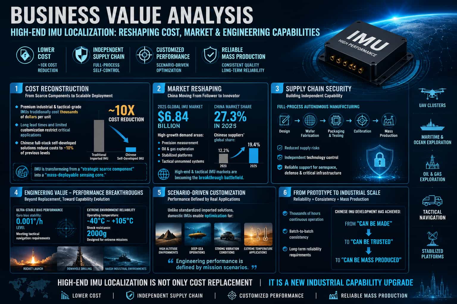
For a long time, procurement channels for high-end MEMS IMUs have been severely limited; users were forced to choose from a handful of international suppliers, accepting standardized off-the-shelf products, enduring long lead times, and paying premium prices. The emergence of localized supply solutions is transforming this landscape. Beyond matching performance benchmarks, domestic IMU suppliers offer differentiated value across four key dimensions, profoundly influencing procurement decisions in the industrial, robotics, and autonomous systems markets. **Cost: From High Premiums to Economic Viability** Cost is the primary driver of supply diversification. The high-end IMU market has long been characterized by concentrated supply and rigid pricing. Domestic suppliers derive their cost advantages from three levels: In manufacturing, advanced processes—such as wafer-level packaging—have significantly improved yields, effectively amortizing the manufacturing cost per chip. Regarding calibration efficiency, fully automated lines utilize batch parallel testing, drastically reducing the time and equipment costs associated with traditional item-by-item calibration. In terms of the supply chain, localizing the entire value chain—from chip design to packaging and testing—minimizes intermediaries, logistics costs, and tariffs. At scale, domestic products can be priced at 50% to 70% of comparable imports, reducing the overall Bill of Materials (BOM) cost by 30% to 60%. For end-users, this translates to superior procurement costs for equivalent performance, as well as a more predictable long-term cost structure. **Delivery: From Months of Waiting to Flexible Scheduling** Long lead times for imported IMUs have long been a pain point. Delivery for high-end MEMS IMUs often takes weeks or even months from the time of order. Global supply chain fluctuations can further extend these timelines or even cause disruptions. The delivery advantages of localized supply manifest in two ways: regarding production capacity, multiple fully automated calibration lines have been established domestically, ensuring capacity planning remains unaffected by the international trade environment. In terms of responsiveness, domestic manufacturers can shorten sample delivery times to just a few days. From component selection and design to debugging and validation, local technical support teams provide full-lifecycle assistance—spanning R&D to mass production—thereby significantly accelerating time-to-market. For development projects with tight schedules, these delivery advantages are often more compelling than price alone. Customization: From Standardization to On-Demand Configuration Imported IMUs are primarily standardized, off-the-shelf products, forcing users to accept fixed specifications. Domestic suppliers have broken this limitation by offering greater customization flexibility: at the hardware level, dimensions, mounting methods, connector types, and supply voltages can be tailored; at the software level, communication protocols, data output formats, and register mappings can be customized; and regarding performance, parameters such as measurement ranges, filtering bandwidths, calibration temperature ranges, and even proprietary error compensation models can be optimized for specific application scenarios. This flexibility is particularly crucial for two types of users: those needing to retrofit existing systems, where customization minimizes system modifications; and those operating under unique conditions, where customization maximizes performance for specific scenarios. Support: From Technical Documentation to System Empowerment In the context of global competition, technical support capabilities are defined not merely by response speed, but by the construction of a technical ecosystem that deeply empowers the user. Regarding comprehensive and internationalized documentation, domestic suppliers provide complete data sheets, application notes, reference designs, and integration guides based on real-world cases in both Chinese and English, ensuring that engineers worldwide can efficiently handle component selection and design. In terms of an open technical ecosystem, domestic suppliers typically provide fully open register manuals, communication protocol stack source code, and calibration toolchains, allowing users to exercise deep control over product behavior without relying on a vendor's closed APIs. This openness offers a distinct value proposition often lacking in imported products, making it particularly suitable for R&D teams with deep system customization needs. Regarding professional support teams, engineers with extensive industry experience assist users with precise selection and solution evaluation during the pre-sales phase, and help resolve complex issues—such as hardware-software integration and data fusion—during the R&D phase. This professional collaboration effectively reduces system integration risks for users and shortens time-to-market. For demanding industrial-grade and automotive-grade applications, comprehensive technical documentation, an open technical ecosystem, and professional technical collaboration collectively ensure high-quality delivery. Conclusion Cost, delivery, customization, and support—these four advantages form a complete value loop: cost advantages lower procurement barriers, delivery advantages ensure project schedules, customization advantages meet differentiated needs, and support advantages eliminate technical obstacles.
Read More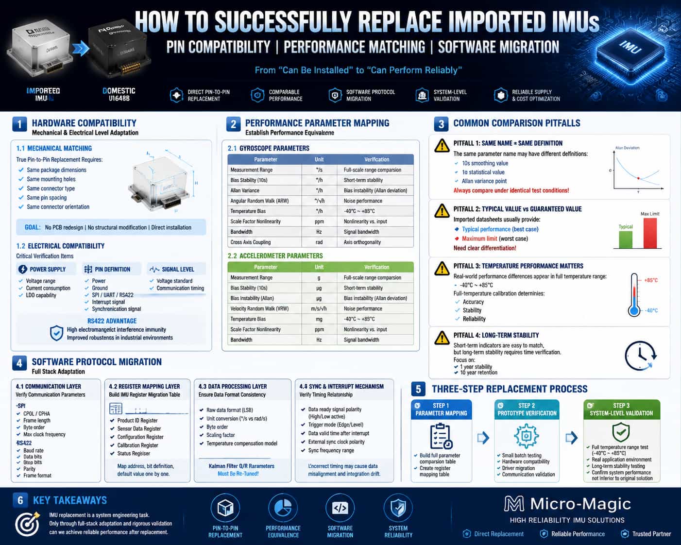
1. Introduction Replacing an Inertial Measurement Unit (IMU) is far more complex than simply swapping out a chip. IMU replacement entails system-level adaptation across multiple layers, including mechanical mounting, electrical connections, communication protocols, register mapping, and data processing pipelines. This article systematically outlines the practical steps and technical considerations involved in the IMU replacement process, focusing on three dimensions: hardware pin compatibility, performance parameter benchmarking, and software protocol migration. 2. Pin Compatibility: Mechanical and Electrical Adaptation 2.1. Mechanical Dimensions and Mounting Interfaces The first level of pin compatibility is mechanical compatibility. High-end IMUs often utilize modular packaging; physical dimensions, mounting hole locations, and connector types directly determine the feasibility of a "drop-in replacement." To achieve replacement without modifying the PCB or housing, these mechanical parameters must match on a 1:1 basis. In practice, key factors to verify include: module dimensions (length, width, height), mounting hole diameters and positions, connector models and pin pitch, and connector orientation and locking mechanisms. While some replacement products feature optimized dimensions beneficial for new designs, these changes can create mounting issues for drop-in replacements in existing systems, potentially necessitating the design of adapter brackets. 2.2. Electrical Pin Definitions and Signal Levels Following mechanical compatibility comes electrical compatibility. Core verification items include: supply voltage and power consumption, pin function definitions (power, ground, communication interfaces, interrupt/synchronization signals), and signal level standards. Taking the SPI interface as an example, some replacement products utilize RS-422 differential interfaces. RS-422 offers common-mode noise rejection exceeding 80 dB—an improvement of 30–40 dB over single-ended signals—which is crucial for system robustness in high-EMI environments (such as industrial motor drives). However, converting between RS-422 and SPI involves redesigning the protocol layer; it is not merely a matter of changing a few wires. 2.3. Power Supply and Timing Considerations Power-up timing and power consumption differences are the most frequently overlooked aspects of pin compatibility. If the replacement product consumes more power than the original, the load capacity of the existing power supply's LDO (Low-Dropout Regulator) must be verified. Differences in power-up initialization timing are also critical; some substitute products may require a longer stabilization time upon power-up, necessitating an added delay in the host controller before data reading begins. Additionally, some modules exhibit pulse noise at the moment of power-up, requiring the addition of filtering capacitors at the power supply input. 3. Parameter Benchmarking: Precise Mapping of Performance Metrics 3.1. Key Dimensions for Parameter Benchmarking The essence of parameter benchmarking is establishing a "performance equivalence relationship" between the substitute product and the original product. Key benchmarking dimensions include: Gyroscope: Measurement range (°/s), bias stability (°/h), bias instability (°/h, Allan variance), angular random walk (°/√h), full-temperature bias (°/h), scale factor nonlinearity (ppm), bandwidth (Hz), and cross-coupling (rad). Accelerometer: Measurement range (g), bias stability (μg), bias instability (μg, Allan variance), velocity random walk (m/s/√h), full-temperature bias (mg), scale factor nonlinearity (ppm), and bandwidth (Hz). 3.2. Key Pitfalls in Benchmarking Pitfall 1: Differing metric definitions. While all may be labeled "bias stability," some manufacturers use a 10-second smoothed value, others use a 1σ statistical value, and some use the inflection point value from the Allan variance plot. Comparisons must be made under identical testing conditions. Pitfall 2: Typical values vs. maximum values. Datasheets for imported products often list both typical and maximum values, whereas substitute products might only specify an upper limit (≤). It is essential to distinguish between "typical performance" and "guaranteed performance" during benchmarking. Pitfall 3: Overlooking full-temperature performance. Benchmarking parameters at room temperature is relatively straightforward; the true performance gap often manifests across the full operating temperature range (-40°C to 85°C). Imported products benefit from factory calibration covering the entire temperature range, a key factor in their superior performance. If substitute products are calibrated only at room temperature, their performance may degrade significantly under extreme temperatures. Pitfall 4: Long-term stability. Short-term metrics found in datasheets are easy to benchmark, but long-term metrics—such as stability over one year or retention over ten years—require time to verify. This represents the most difficult "engineering maturity barrier" for substitute products to overcome. 4. Software Protocol Porting: Full-Stack Adaptation from Physical to Application Layers Software porting is the most complex and frequently underestimated aspect of IMU replacement. Even if pinouts and parameters are perfectly matched, the system will fail to operate if the software layers are incompatible. 4.1. Communication Protocol Layer First, the communication interface type—SPI, I2C, UART, or RS422—and its specific parameters must be verified. Taking SPI as an example, parameters to check include clock polarity (CPOL) and clock phase (CPHA), frame length (8/16/32-bit), data byte order (big-endian/little-endian), and maximum clock frequency. In SPI communication, the "inter-transfer delay"—the minimum interval between two SPI commands—must be handled correctly to avoid data read failures. For RS422, parameters such as baud rate, data bits, stop bits, parity bits, and frame format require verification. 4.2. Register Mapping Layer This is the core challenge of software porting. It is virtually impossible for IMUs from different manufacturers to align perfectly regarding register address allocation, data formats, and control bit definitions. Key register categories requiring porting include: product identification registers (for verifying the communication link), sensor data registers (addresses and bit widths may differ), configuration registers (measurement range, filtering, sampling rate), calibration registers (addresses for bias and scale factor correction), and status registers (bit definitions for error flags and data-ready flags). In practice, a "register mapping table" should be created to map the address, bit definitions, and default values of each key register from the original product to the replacement product. For functions that do not exist in the replacement, adaptations must be made at the driver layer, or relevant calls must be removed. 4.3. Data Processing Layer Differences may exist in the raw output format of sensor data (LSB vs. physical units), units of measurement (°/s vs. rad/s), byte order, and scaling factors. If the replacement product outputs physical quantities directly while the original product outputs raw LSB values, a unit conversion interface must be added to the driver layer. Error compensation models may also differ; for instance, imported products might feature built-in first-order polynomial compensation, whereas the replacement product might support higher-order temperature compensation models, necessitating an expansion of the compensation interface. The Q and R noise matrices for the Kalman filter must be recalibrated based on the stochastic walk characteristics of the replacement product; the original parameters cannot be reused directly. 4.4. Synchronization and Interrupt Mechanisms Parameters such as the polarity (active high/low), trigger mode (edge/level), and timing relationship (latency between the data-ready signal and valid data) of the data-ready signal may vary. The polarity and frequency range of the external synchronization clock must also be verified. Improper handling can lead to timing mismatches in data acquisition and cumulative errors in attitude estimation. 5. Conclusion IMU replacement is a systematic engineering task, far more complex than a simple "pin-to-pin" component swap. At the hardware level, full compatibility regarding mechanical dimensions, pin assignments, and power-up sequencing must be verified. At the parameter level, a point-by-point comparison under identical test conditions is required, with particular attention paid to performance across the full temperature range and long-term stability. At the software level, full-stack adaptation is necessary, covering everything from communication protocols and register mapping to data processing pipelines. In practice, a "three-step" strategy is recommended: first, establish a comprehensive parameter comparison list and register mapping table; second, conduct hardware compatibility verification and driver porting using a small batch of samples; and third, perform system-level performance validation across the full temperature range and under actual operating conditions to confirm that the system's overall performance with the replacement component is not inferior to the original solution. Only through this process can one successfully transition from merely "fitting the part" to achieving "optimal system performance."
Read More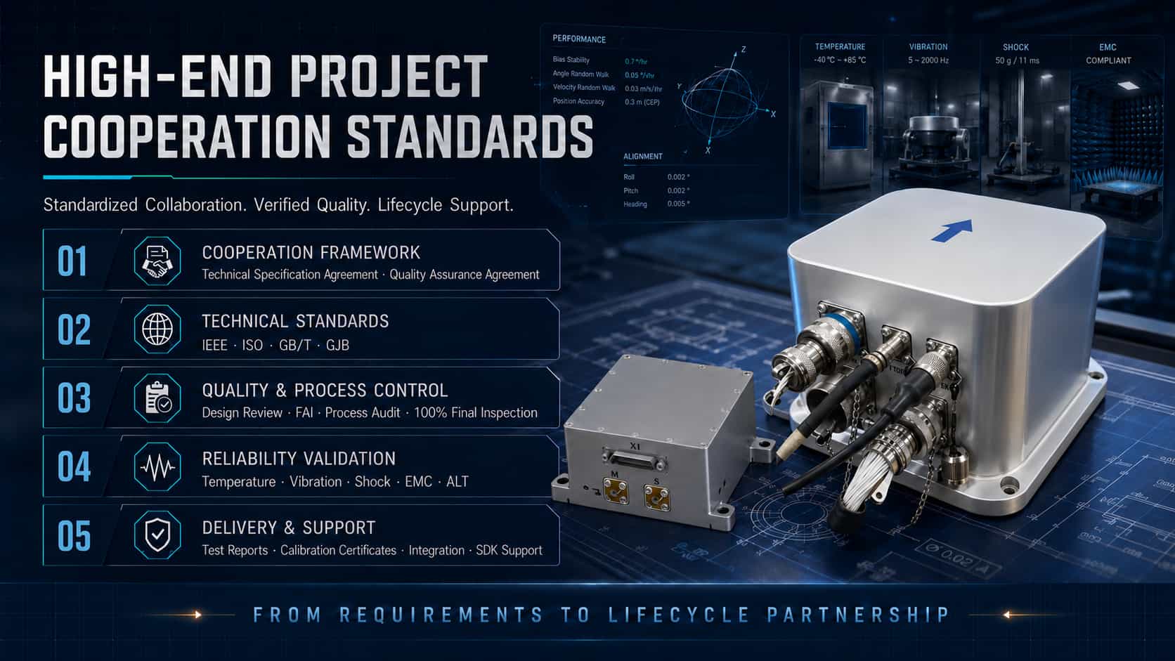
Inertial sensors—including accelerometers, gyroscopes, and inertial measurement units (IMUs)—are core components of aviation navigation, guidance, and control systems; their performance and reliability directly determine flight safety and mission success. Projects involving inertial sensors in the aviation sector entail full lifecycle management, ranging from qualification and certification, delivery and acceptance, and custom R&D to technical support. This article provides a technical analysis of these four dimensions, drawing upon international standard systems and engineering practices. 1. Aviation Project Qualification To enter the airworthy market, aviation inertial sensors must undergo a series of rigorous qualification and certification processes. These cover multiple aspects, including hardware environmental adaptability, software safety, hardware design assurance, and technical standard verification. Environmental Adaptability Certification: RTCA DO-160, *Environmental Conditions and Test Procedures for Airborne Equipment*, is the core standard for environmental testing of avionics hardware and is recognized by the International Organization for Standardization (ISO) as the de facto international standard ISO-7137. This standard defines minimum environmental test conditions and procedures for a full range of airborne equipment, spanning everything from light general aviation aircraft and helicopters to large jetliners and supersonic aircraft. DO-160 encompasses over 20 tests, including temperature, vibration, shock, humidity, altitude, waterproofing and dustproofing, salt fog and fungus resistance, electromagnetic compatibility (EMI/EMS), lightning effects, electrostatic discharge, and power input and voltage transients. Software and Hardware Certification: DO-178, *Software Considerations in Airborne Systems and Equipment Certification*, is the gold standard for aviation software safety certification. It categorizes software into assurance levels ranging from A to E, with Level A applying to the most critical flight safety functions. DO-254, *Design Assurance Guidance for Airborne Electronic Hardware*, addresses design assurance for complex electronic hardware. Certification for inertial navigation products typically requires software to meet DO-178B/C Level A standards and hardware to meet DO-254 Level A standards. Technical Standard Order (TSO): A TSO is a minimum performance standard issued by the U.S. Federal Aviation Administration (FAA); manufacturers must obtain TSO Authorization (TSOA) before their equipment can be installed on certified aircraft. TSOs related to inertial navigation systems include TSO-C4c (Gyroscopes), TSO-C5f (Attitude and Heading Reference Systems), TSO-C6e (Directional Gyros), TSO-C88b (Autopilots), and TSO-C201 (AHRS), among others. GJB References: Qualification for Chinese military inertial sensor projects is primarily based on the GJB 9001C quality management system, the qualification review for equipment manufacturing units, and the GJB 150 series of environmental test standards; technically, these share a common lineage with MIL-STD and DO series standards. 2. Delivery Specifications Delivery specifications for inertial sensors cover product inspection, acceptance criteria, packaging and transportation, and documentation delivery, ensuring quality control and traceability throughout the entire process from factory departure to aircraft installation. Inspection and Acceptance: Delivery inspections for aviation-grade inertial sensors are categorized into factory inspection (full-parameter performance testing and full-temperature calibration), acceptance inspection (re-testing upon arrival), and qualification inspection (type-certification testing). Specifications for airborne inertial navigation systems cover technical requirements, test methods, inspection rules, and packaging/transportation; specifications for civil UAV IMUs detail classification levels and maintenance requirements. Packaging and Transportation: Packaging for military inertial navigation equipment follows MIL-STD-2073-1 (Military Level B individual packaging), specifying methods to prevent corrosion and mechanical damage to ensure integrity during storage and multiple transport cycles; marking complies with MIL-STD-129. Civil aviation applications refer to DO-160 and related specifications, outlining specific requirements for moisture, shock, and electrostatic protection. Documentation Delivery: Deliverables typically include product specifications, test reports (environmental testing, electromagnetic compatibility, life testing, etc.), calibration certificates, Declarations of Conformity (DoC), user manuals, and maintenance manuals. For products certified under DO-178/DO-254, a complete software/hardware design assurance data package is also required. 3. Custom Development Aviation applications often demand highly customized inertial sensors; different platforms (fixed-wing aircraft, rotorcraft, UAVs) and mission profiles (civil aviation, military, scientific research) impose varying requirements regarding accuracy, size, weight, power consumption (SWaP), interface protocols, and environmental adaptability. Hardware Customization: Custom development encompasses sensor selection and configuration (choosing between technologies such as MEMS, fiber-optic, or laser gyros), customization of form factors and mechanical interfaces (e.g., modifying the housing to fit specific installation spaces), connector selection (e.g., MIL-Spec 38999 filtered connectors), and design enhancements for environmental resilience (vibration and shock resistance, wide operating temperature range). Software and Algorithm Customization: This includes the customization of communication protocols (RS-232/422/485, ARINC, CAN, etc.), configuration of data output formats and rates, optimization of sensor fusion algorithms, and programming for lever-arm effects and mounting orientation. Some suppliers also offer custom development of non-standard testing systems and specialized software tools. Customization Process: A typical custom development workflow involves requirements analysis, solution design, prototype fabrication, environmental verification (e.g., DO-160 testing), system integration, and flight testing. Many suppliers possess end-to-end in-house manufacturing capabilities—ranging from MEMS wafer fabrication to IMU calibration—ensuring quality control for customized products. 4. Technical Support Technical support is a crucial component of the full lifecycle service for inertial sensors, covering the entire chain from selection consultation and system integration to on-site commissioning, fault diagnosis, and maintenance/calibration. Selection and Integration Support: Suppliers typically provide evaluation kits to help customers verify performance during the early stages of a project. Technical teams assist customers throughout the process—from sensor selection and interface matching to system integration—resolving engineering challenges such as data fusion, coordinate system transformation, and error compensation. Some manufacturers offer 24/7 technical support covering the entire workflow, from selection and integration to data fusion. Calibration and Maintenance Services: Inertial sensors require periodic calibration after prolonged use to compensate for bias drift and scale factor variations. Suppliers holding aviation certifications (such as EASA Part 21G and EN9100 quality management systems) can provide calibration and maintenance services that meet aviation standards. Some manufacturers also provide MTBF (Mean Time Between Failures) data. Full-lifecycle partnership: Leading inertial sensor suppliers offer more than just standard products; they establish partnerships that span the entire product lifecycle—from conceptual design, prototyping, and airworthiness certification support to mass production delivery and long-term maintenance. This model reduces project risk and shortens R&D cycles for customers while ensuring the sustained reliability of aviation inertial sensors in demanding operational environments. 5. Conclusion Aviation applications for inertial sensors have established a comprehensive system covering everything from certification (DO-160/DO-178/DO-254/TSO) and delivery specifications (MIL-STD-2073 packaging and acceptance inspection) to custom R&D (flexible hardware/software adaptation) and technical support (full-lifecycle services). Understanding and effectively leveraging this multi-layered framework of standards and services is essential for the successful application of inertial sensors in aviation projects.
Read More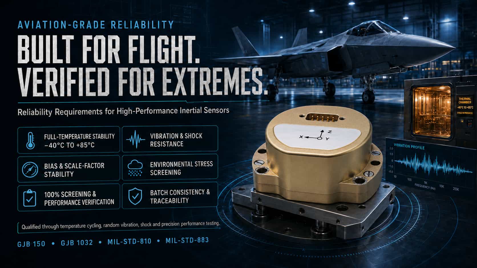
Inertial sensors—including accelerometers, gyroscopes, and inertial measurement units (IMUs)—are core components of navigation, guidance, and control systems in the aviation, aerospace, maritime, and defense sectors; their environmental adaptability and long-term reliability directly determine the operational effectiveness of weapon systems. Military-grade inertial sensors must undergo rigorous Environmental Stress Screening (ESS), where the application of appropriate environmental stresses—such as thermal and mechanical loads—accelerates the manifestation of latent internal defects into failures, allowing for their subsequent elimination. In the international defense and aerospace industries, a comprehensive testing and verification framework for inertial sensors has been established, based on standards such as the US military standards (MIL-STD), ISO, IEEE, and the avionics standard RTCA DO-160. This article examines three key testing categories—high/low-temperature cycling, vibration/shock, and aging screening—analyzing them from the perspectives of both standard frameworks and technical essentials. 1. High/Low-Temperature Cycling Test High/low-temperature cycling tests aim to evaluate the performance stability and structural integrity of inertial sensors when subjected to alternating extreme temperatures. Temperature fluctuations can cause drift in critical parameters—such as sensor bias and scale factor—thereby affecting overall system accuracy. International Standards: MIL-STD-810 outlines procedures for high- and low-temperature exposure tests, covering both operational and storage conditions. Within MIL-STD-883, Method 1010 (Temperature Cycling) specifies "Condition B"—ranging from -55°C to 125°C with up to 100 cycles—while Method 1011 details thermal shock testing procedures. In the avionics sector, Section 5 of RTCA DO-160 specifically regulates temperature variation test procedures. Additionally, ISO 16063-34:2019 specifies sensitivity testing methods at fixed temperatures from the perspective of sensor calibration, covering a range from -190°C to 800°C. Technical Essentials: Key parameters for temperature cycling tests include the temperature range (e.g., -55°C to +85°C or +125°C), rate of temperature change, dwell time, and the number of cycles. In practical testing, conditions typically involve a temperature range of -55°C to +85°C, a 30-minute dwell time, and a temperature change rate of 5–10°C/min. Selecting the appropriate rate is critical: an excessively high rate may exceed the device's thermal inertia limits, leading to false failures, while an excessively low rate may fail to effectively reveal defects. Regarding performance evaluation, parameters such as bias stability and scale factor repeatability must be measured after cycling; for instance, a specific inertial navigation system requires the attitude angle output error to be ≤0.15° across the -55°C to +85°C range. MIL-STD-810 emphasizes tailoring test profiles based on the platform type (e.g., fixed-wing aircraft, rotorcraft, vehicles). 2. Vibration and Shock Testing Vibration and shock tests simulate the mechanical environments experienced by inertial sensors during launch, flight, landing, and transportation, verifying their structural integrity and output accuracy under dynamic loads. International Standards: MIL-STD-810 Method 514 (Vibration) and Method 516 (Shock) serve as the core standards in this field. Method 514.7 specifies procedures and spectral density requirements for random vibration testing (e.g., 25 grms, 10-hour random vibration test). MIL-STD-202 Method 213 outlines mechanical shock test procedures (e.g., 50 g, 11 ms half-sine pulse). The ISO 16063 series provides the methodological basis for vibration and shock sensor calibration: Part 21 covers vibration calibration via reference sensor comparison; Part 22 covers shock calibration; and Part 43 covers accelerometer calibration based on model parameter identification. RTCA DO-160 Section 8 covers sinusoidal and random vibration in the 5 Hz to 2000 Hz range. Technical Highlights: Vibration testing generally encompasses two modes: sinusoidal sweep and random vibration. The power spectral density for random vibration must be tailored to the platform type—for example, requiring a spectral density of 0.04 g²/Hz across the 20 Hz to 2000 Hz range. Shock testing typically employs half-sine pulses, with characteristic parameters including peak accelerations of 50–400 g and durations of 2–35 ms. During testing, the sensor output must be monitored in real-time under vibration or shock conditions, with particular attention paid to anomalies such as zero-bias drift, scale factor variations, and signal interruptions. MIL-STD-810 emphasizes that test severity levels should be based on measured environmental data rather than arbitrary selection; this "data-driven" approach warrants close attention in engineering practice. 3. Aging Screening Tests Aging screening (also known as Environmental Stress Screening, or ESS) is a critical process that uses accelerated environmental stress to eliminate products prone to early-life failure and ensure batch consistency. International Standards: MIL-STD-883 Method 1010 (Temperature Cycling) is the core method for component-level screening and is frequently combined with random vibration testing. Industry practices often employ screening conditions such as 250 cycles, a temperature range of -40°C to 85°C, and a 73-minute dwell time. MIL-STD-810 specifies methods for applying combined stresses from a system-level environmental testing perspective. Although RTCA DO-160 focuses on airworthiness certification, its environmental test procedures also serve as a valuable reference for screening aviation-grade sensors. The Arrhenius model is widely used internationally to predict service life during Accelerated Life Testing (ALT). China’s GJB 1032A-2020 aligns closely with MIL-STD-883 regarding screening philosophy, though specific requirements for cycle counts and temperature change rates differ (e.g., GJB commonly specifies a rate of 15°C/min). Technical Highlights: Aging screening exposes latent defects (such as solder joint cracks, chip delamination, or broken bond wires) through a combination of "temperature acceleration" and "vibration excitation." Temperature change rates are typically set between 5°C/min and 15°C/min, while dwell times are sufficient to ensure device temperature stabilization (usually 30–60 minutes). Screening stress levels must remain within the product's design strength limits to ensure defects are effectively triggered without inducing irrelevant failure modes. For high-reliability inertial devices, Accelerated Life Testing can be used to compress years of operational stress into a few weeks, allowing for service life extrapolation via modeling. During the screening process, full-parameter testing (covering zero bias, scale factor, threshold, etc.) is required for every device to ensure batch consistency. Conclusion High-low temperature cycling, vibration/shock testing, and burn-in screening each play distinct yet complementary roles: temperature cycling evaluates zero-bias stability and structural fatigue resistance under extreme temperature fluctuations; vibration and shock testing verify output accuracy and mechanical integrity under dynamic loads; and burn-in screening exposes latent defects—such as solder joint cracks or chip delamination—through accelerated stress, thereby ensuring product reliability at the batch level. Three points require attention in practical application: first, the precision of the test equipment should be at least three times finer than the tolerance of the parameter being measured to ensure reliable results; second, test conditions must be appropriately tailored to the specific platform type (e.g., fixed-wing aircraft, rotorcraft, vehicles, or ships) rather than blindly applying generic standards, which could lead to over-testing or under-testing; and third, standards should be integrated and applied flexibly—MIL-STD provides a general environmental framework, ISO offers calibration methodologies, IEEE supplies sensor testing protocols, and DO-160 outlines specific airworthiness requirements. Only by thoroughly understanding the scope of each standard and effectively combining them can the reliable operation of inertial sensors in harsh environments be guaranteed.
Read More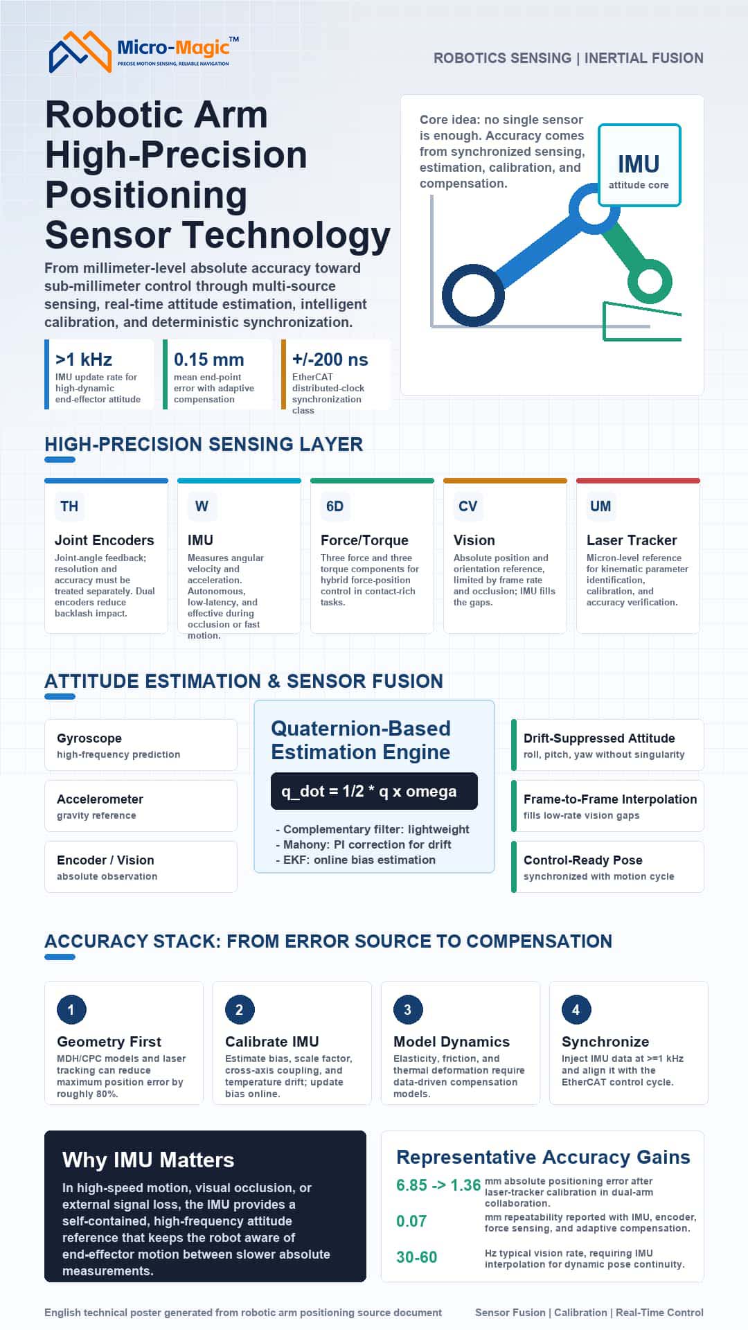
Introduction The absolute positioning accuracy of robotic arms—transitioning from the millimeter to the sub-millimeter scale—is constrained by multiple error sources: geometric parameter deviations (accounting for over 80%), sensor drift, elastic deformation, and communication jitter. Relying on single-sensor inputs or purely kinematic control is insufficient to meet the demands for dynamic, high-precision performance. Particularly during high-speed motion or in scenarios involving visual occlusion, the IMU—characterized by high-frequency operation, autonomy, and zero latency—serves as a cornerstone for pose estimation. Current technological trends favor a combination of multi-source sensor fusion, intelligent calibration, and high-real-time synchronization. High-Precision Positioning and Sensing Technologies Joint Encoders Encoders determine the accuracy of joint angle feedback. Key metrics: resolution and accuracy must not be conflated. Optical encoders can achieve an accuracy of 5 arcseconds and 23-bit resolution; magnetic encoders offer robust resistance to contaminants; and high-end systems employ dual-encoder setups to eliminate the effects of backlash. Inertial Measurement Units (IMUs)—The Core of Pose Estimation IMUs integrate tri-axial gyroscopes and accelerometers to directly measure the angular velocity and linear acceleration of the end-effector. Gyroscope integration yields relative pose data with update rates exceeding 1 kHz—far surpassing vision systems—while accelerometers provide an absolute gravity reference during static states to calibrate integration drift. However, IMUs suffer from gyroscope integration drift (which can reach 30° after 10 minutes of inactivity) and accelerometer motion noise; resolving these issues is the central challenge addressed by sensor fusion. The unique advantage of the IMU lies in its independence from external signals and immunity to occlusion or latency-induced jitter, making it an irreplaceable autonomous sensor for high-frequency pose sensing at the robotic arm's end-effector. Six-Axis Force Sensors These sensors simultaneously measure three force components and three torque components, enabling hybrid force/position control. With an accuracy of 0.5% and repeatability error of 0.1%, they are utilized in contact-based tasks such as precision assembly and grinding. Vision Systems Configured as either "eye-in-hand" or "eye-to-hand," binocular vision systems can achieve positional accuracy of 1.2 mm and orientation accuracy of 0.15°, though they are limited by refresh rates (30–60 Hz) and occlusion issues. IMUs can be used to perform high-frequency pose interpolation between visual frames. External Calibration Equipment A laser tracker (offering micron-level accuracy) serves as the reference tool for kinematic calibration, parameter identification, and accuracy verification. Attitude Estimation and Sensor Fusion Attitude Representation Methods Euler angles are intuitive but suffer from the gimbal lock problem; degrees of freedom are lost when the pitch angle θ = ±90°. Quaternions: q = q₀ + q₁i + q₂j + q₃k, satisfying q₀² + q₁² + q₂² + q₃² = 1. Rotation operation: p' = qpq⁻¹ Quaternions are singularity-free and allow for smooth interpolation, making them the standard attitude representation in modern robotic systems. The core of IMU attitude estimation lies in solving the quaternion differential equation. Fundamentals of IMU Attitude Estimation: Quaternion Differential Equation Updating the quaternion using angular velocity ω = [ωₓ, ωᵧ, ωᵨ]ᵀ: q̇ = ½ q ⊗ ω Discretization (first-order integration): qₖ₊₁ = qₖ ⊗ (cos(‖ω‖Δt/2), (ω/‖ω‖)sin(‖ω‖Δt/2)) This equation forms the basis for all IMU-based attitude estimation algorithms. Complementary Filtering and the Mahony Algorithm Complementary filtering fuses gyroscope integration (reliable at high frequencies) with accelerometer data (reliable at low frequencies): θ(t) = α·θ_gyro(t) + (1-α)·θ_acc(t) (α typically ranges from 0.98 to 0.995) The Mahony filter introduces PI closed-loop correction: gyroscope drift is compensated using an error term *e*—derived from the cross product of the accelerometer measurement *a_m* and the gravity reference *g_ref*—where *e* = *a_m* × *g_ref* and *ω_corr* = Kₚ*e* + Kᵢ∫*e*dt. This method is computationally efficient and widely used in embedded systems for real-time attitude estimation of IMUs mounted on robotic arm end-effectors. Extended Kalman Filter (EKF)—Optimal Fusion Framework The EKF uses gyroscope integration for prediction and accelerometer data (along with magnetometer and encoder-based forward kinematics) for observation. The state vector is defined as x = [qᵀ, b_gᵀ]ᵀ (attitude quaternion + gyroscope bias). Prediction: $\dot{\hat{x}} = f(\hat{x}, \omega_m - b_g)$, $P = FPF^T + Q$ Update (using accelerometer observations of the gravity vector): $K = PH^T (HPH^T + R)^{-1}$ $\hat{x}^+ = \hat{x} + K(z - h(\hat{x}))$ The EKF enables online estimation of gyroscope bias, significantly suppressing long-term drift. A tightly coupled EKF integrating IMU data with encoders or vision systems is the standard architecture for achieving high-precision pose estimation of robotic arm end-effectors. Multi-source Fusion Strategy Heterogeneous sensors are fused at the data, feature, or decision level. As a high-frequency internal sensor, the IMU is often combined with encoders (low-frequency, high-precision angular data), vision systems (absolute position but low frame rate), and 6-axis force sensors (contact information) to form either loosely or tightly coupled systems. Hybrid fusion is currently the mainstream approach for achieving micron-level precision, with the IMU providing an indispensable real-time reference. Error Analysis and Calibration Compensation Dominance of Geometric Errors The classical DH model relies on idealized assumptions. Extended models (such as MDH and CPC) introduce additional geometric parameters. Calibration using a laser tracker can reduce maximum positional error by approximately 80%. IMU Error Calibration MEMS IMUs require calibration for bias, scale factors, cross-coupling, and temperature drift. Accelerometers are typically calibrated using the factory six-position method, while gyroscopes are calibrated using rate turntables. In robotic arm systems, kinematic constraints (such as static phase detection) can be utilized to update IMU bias online, effectively suppressing integration drift. Laser Tracker Calibration Process The robot traverses a set of predefined points while the laser tracker records end-effector coordinates; kinematic parameter deviations are then identified and compensated for. Following calibration, the absolute positioning accuracy of the dual-arm collaborative robot improved from 6.85 mm to 1.36 mm. Non-geometric Errors and Dynamic Compensation Non-geometric factors—such as joint elasticity, thermal deformation, and friction—cannot be adequately described by traditional models. Data-driven calibration methods (e.g., neural networks, Gaussian processes) enable the learning of error mappings from measured data. Compensation models integrating IMUs, encoders, and six-axis force sensors, combined with adaptive control, can reduce the mean end-effector positioning error to 0.15 mm and achieve a repeatability of 0.07 mm. Real-time Communication and Multi-axis Synchronization Multi-axis coordination requires the deterministic transmission of control commands. The EtherCAT industrial Ethernet bus employs an "on-the-fly processing" mechanism; its Distributed Clock (DC) synchronization error is as low as ±200 ns, with a jitter of ±5 μs. IMU data must be fed into the master controller at a rate of ≥1 kHz via high-bandwidth interfaces (such as SPI) and aligned with EtherCAT cycles to ensure strict frequency synchronization between attitude fusion and motion control. Trends and Conclusions High-precision robotic arm positioning is evolving toward a paradigm of multi-modal sensing, AI-based dynamic compensation, and real-time edge computing. As the core component for high-frequency, autonomous attitude sensing, the IMU—deeply integrated with encoders, vision systems, and force sensors—will play an increasingly indispensable role in high-speed, highly dynamic scenarios. Achieving absolute positioning accuracy at the sub-millimeter or even micron level requires coordinated optimization across four layers: sensing, computation, calibration, and synchronization.
Read More
Current mainstream technical approaches for inertial navigation systems fall into two categories: MEMS-based inertial navigation (utilizing Micro-Electro-Mechanical Systems) and fiber-optic inertial navigation (based on optical interference principles). These two technologies differ fundamentally in their physical principles, performance metrics, cost structures, and application scenarios. This article provides a comprehensive, multidimensional comparison of these technologies to assist engineers in making informed decisions during the selection process. I. Fundamental Differences in Operating Principles MEMS inertial navigation systems employ silicon micromachining technology to fabricate movable micro-masses on a chip; when the carrier moves, inertial forces cause these masses to displace, generating electrical signals via capacitance changes—a fully solid-state design with no rotating parts. Fiber-optic inertial navigation systems rely on the Sagnac effect, where a laser beam is split into two beams propagating in opposite directions within a fiber-optic coil; carrier rotation creates an optical path difference between the beams, and angular velocity is calculated through interference detection. Sensitivity increases with the length of the fiber coil. These differences in principle dictate the inherent characteristics of each technology: MEMS systems function as "solid-state mass" sensors—insensitive to vibration but limited by manufacturing precision—whereas fiber-optic systems act as "optical interferometers," capable of high precision but significantly influenced by fiber length and temperature. II. Comparison of Core Performance Parameters Bias stability is the primary metric for measuring inertial navigation accuracy. Typical values for MEMS inertial navigation range from 0.5°/h to 10°/h; while high-end tactical-grade products can achieve 0.05°/h to 0.1°/h, they are approaching the technology's precision ceiling. In contrast, fiber-optic inertial navigation systems typically exhibit bias stability between 0.01°/h and 0.1°/h, with high-end products reaching 0.001°/h (arc-second level). Fiber-optic systems demonstrate a clear advantage in scenarios requiring pure inertial navigation over durations ranging from several minutes to tens of minutes. Angle random walk reflects the impact of white noise on attitude integration. Typical values for MEMS inertial navigation range from 0.1°/√h to 0.5°/√h, whereas fiber-optic systems can achieve values as low as 0.001°/√h to 0.01°/√h. This means that during short-term dynamic maneuvers, the attitude output from fiber-optic inertial navigation systems is smoother and exhibits less jitter. Scale factor nonlinearity: For MEMS inertial navigation systems, this typically ranges from 0.1% to 1%, whereas fiber-optic systems can achieve 0.001% to 0.01%. This nonlinearity advantage is crucial for high-dynamic maneuvers (such as those performed by missiles or fighter jets). Full-temperature bias error: MEMS silicon materials have high temperature coefficients; without compensation, the thermal drift of MEMS inertial systems can reach tens or even over a hundred °/h/°C. Modern high-end MEMS products utilize integrated temperature compensation and polynomial fitting to reduce thermal drift to within 1°/h/°C. Fiber-optic systems are also temperature-sensitive, but the temperature coefficient of the fiber coil itself can be partially mitigated through symmetrical winding techniques; combined with precise temperature control, the full-temperature error can be kept below 0.01°/h/°C. Vibration rectification error: MEMS inertial systems are prone to DC drift under high-frequency, intense vibration—an inherent flaw. Fiber-optic systems, lacking moving proof masses, exhibit excellent vibration resistance, maintaining accuracy far better than MEMS systems in vibrating environments. Startup time and response characteristics: MEMS inertial systems output data immediately upon power-up, with startup times in the millisecond range. Fiber-optic systems require a warm-up and stabilization period (typically ranging from tens of seconds to several minutes) because the light source and fiber coil must reach thermal equilibrium; otherwise, significant zero-point drift occurs. III. Cost Structure and Price Range MEMS inertial systems benefit from large-scale semiconductor manufacturing processes, resulting in very low unit costs. Prices range from $3–$15 for consumer-grade MEMS IMU chips, $100–$500 for industrial-grade modules (featuring temperature compensation and calibration), and approximately $1,000–$3,000 for tactical-grade MEMS inertial systems (including algorithms). The cost of fiber-optic inertial systems is primarily driven by the fiber coil, precision winding processes, the light source (SLD), and the photodetector. Fiber coils require high-precision winding, entailing high labor and equipment costs, and—unlike chips—cannot benefit from the same economies of scale to drive down prices. Low-precision fiber-optic gyroscope (FOG) modules (bias stability in the 1°/h range) are priced at approximately $2,000–$5,000; medium-precision units (0.1°/h range) cost about $8,000–$20,000; and high-precision units (0.01°/h range or better) can exceed $50,000–$100,000. Regarding cost structure, MEMS devices have extremely low marginal costs, making them suitable for mass deployment; conversely, fiber-optic inertial navigation systems (INS) have high per-unit costs, though their performance ceiling far exceeds that of MEMS. IV. Size, Weight, and Power Consumption High-precision industrial MEMS INS units typically feature a miniature modular design, often measuring just 30–60 mm on a side. Their compact structure—free of redundant optical components—allows for direct integration into wind turbine platforms or small host equipment with minimal installation footprint. In contrast, fiber-optic INS units incorporate fiber coils, laser sources, optical demodulation circuits, and thermal control structures; consequently, they generally measure 100–200 mm, occupy 5–10 times the volume of MEMS units, require significant installation space, and are unsuitable for integration into compact equipment. MEMS INS units utilize silicon-based MEMS technology, keeping the total weight generally between 20 g and 80 g. This ultra-light weight imposes no additional load on offshore floating platforms or lightweight mounting structures, making them ideal for lightweight installations and stress-free mounting. Fiber-optic INS units, however, feature complex optical structures and heavy metal housings and thermal insulation components, resulting in a total weight of 500–2,000 g. This substantial weight limits their use to heavy, fixed platforms and renders them unsuitable for monitoring scenarios requiring lightweight designs or strict load constraints. MEMS inertial navigation systems are driven by chip-based circuitry and operate with extremely low power consumption—typically just 0.3 to 2 W in a steady state. They support long-term battery operation and continuous (24/7) low-power monitoring, making them ideal for lightweight equipment deployed in remote field or open-ocean environments lacking a continuous power supply. In contrast, fiber-optic inertial navigation systems require continuous power for the laser source, optical signal demodulation, and temperature control modules. Their baseline operating power generally ranges from 10 to 30 W—dozens of times higher than that of MEMS systems—and they require auxiliary heat dissipation structures, limiting their use to fixed engineering platforms with stable mains power and ample power capacity. V. Environmental Adaptability and Reliability MEMS inertial navigation systems are all-solid-state devices with no moving parts, offering high theoretical reliability. However, under conditions of high shock (>10,000g) and intense vibration, the silicon proof mass may stick or fracture. Military-grade MEMS units, featuring specialized packaging, can withstand shocks of up to 20,000g. Their standard operating temperature range is -40°C to 85°C, which can be extended to -55°C to 125°C through screening. Fiber-optic inertial navigation systems also lack moving parts; since the fiber-optic coil is essentially made of glass fiber, it offers superior shock and vibration resistance compared to MEMS. However, the coil is sensitive to bending and stress, and improper packaging can lead to increased optical loss. Fiber-optic systems offer a higher ceiling for environmental adaptability, making them suitable for extreme conditions such as deep-sea submarine pressure, continuous ship motion, and high-G launch environments. Summary of Comprehensive Comparison MEMS inertial navigation systems excel in terms of size, weight, power consumption, cost, and startup speed, but lag behind in maximum achievable accuracy and resistance to vibration-induced drift. Fiber-optic systems excel in ultra-high accuracy, long-term stability, and resistance to environmental interference, but are less competitive regarding size, power consumption, cost, and startup time. There is no "right" or "wrong" choice—only the question of suitability: first determine accuracy requirements, then consider environmental constraints, and finally evaluate the economic factors.
Read More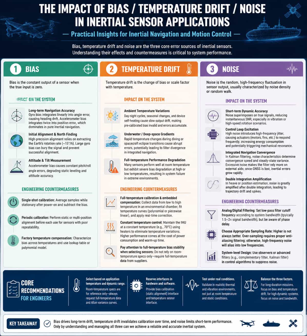
In inertial navigation and motion control projects, sensor bias, thermal drift, and noise are the three core error sources affecting system performance. The following section outlines their manifestations, impact on the system, and mitigation strategies from an engineering perspective. 1. Bias Bias refers to the constant static output of a sensor under zero-input conditions. In engineering applications, bias directly affects long-term integration accuracy and alignment capabilities: · Long-term navigation accuracy: Gyroscope bias accumulates linearly into angular error through integration; the higher the bias, the faster the heading drift. Accelerometer bias translates into position error through double integration, becoming a primary error source—particularly in pure inertial dead reckoning without external corrections. · Initial alignment and north-seeking: High-precision north-seeking requires extracting the north-pointing component from the Earth's angular velocity (approx. 15°/h); if gyroscope bias is excessive, the signal is overwhelmed, rendering effective alignment impossible. · Attitude and tilt measurement: Accelerometer bias directly causes constant offsets in pitch and roll angles, affecting static horizontal attitude accuracy. Engineering mitigation: · Single-event calibration/compensation: Perform static sampling and averaging after power-up, then subtract the constant offset value. · Periodic calibration: For sensors with poor repeatability, perform static-base or indexing alignment before each use. · Factory-level thermal compensation: Record bias values at various temperatures to establish lookup tables or polynomial models. 2. Thermal Drift Thermal drift refers to the variation in sensor bias or scale factor caused by temperature changes. In wide-temperature operating environments, errors induced by thermal drift are often one to two orders of magnitude larger than room-temperature bias: · Ambient temperature fluctuations: Diurnal temperature variations, seasonal changes, and equipment self-heating cause slow drift in sensor output, invalidating pre-calibrated bias values and leading to the accumulation of integration errors over time. · Underwater/deep-space temperature gradients: Rapid temperature changes—such as when a vehicle dives or a spacecraft enters/exits a shadow zone—can cause abrupt errors due to thermal drift, potentially leading to divergence in integrated navigation filters. Performance degradation across the temperature range: Many sensors exhibit excellent specifications at room temperature, but their zero-bias performance deteriorates significantly at high or low temperatures, potentially causing total system failure in extreme environments. Engineering countermeasures: · Full-temperature calibration + embedded compensation: Sensor output is captured in real-time within a thermal chamber across the operating temperature range; a temperature curve (polynomial or piecewise linear) is fitted, and the chip or navigation computer applies real-time corrections based on the current temperature. · Constant temperature control: In high-end applications (such as strategic-grade inertial navigation systems), heaters maintain the IMU at a constant temperature (e.g., 70°C) to eliminate temperature fluctuations, albeit at the cost of increased power consumption and longer startup times. · Prioritizing full-temperature zero-bias stability during selection: Many suppliers provide only room-temperature specifications—which can be misleading for a project—so it is essential to demand full-temperature performance data. 3. Noise Noise refers to random, high-frequency fluctuations in the sensor output, typically characterized by random walk coefficients or noise density. Its impact is primarily observed in short-term dynamics and system stability: · Short-term dynamic accuracy: Noise superimposed on the true signal reduces the instantaneous signal-to-noise ratio (SNR), an effect particularly pronounced during vibration or high-speed rotation. · Control loop excitation: High noise levels introduce high-frequency jitter, causing actuators (such as motors or control surfaces) to respond frequently; this increases energy consumption and may trigger mechanical resonance. · Integrated navigation convergence: In Kalman filtering, noise characteristics determine the convergence rate and steady-state variance of state estimates; excessive noise forces the filter to rely more heavily on external aiding data, meaning that if GNSS lock is lost, pure inertial errors will grow rapidly. · Double-integration amplification effect: In heave measurement or dead reckoning, noise is drastically amplified after double integration, resulting in trajectory drift or signal spikes. Engineering countermeasures: · Analog/digital filtering: Low-pass filter cutoff frequencies are set based on system bandwidth (typically 1.5 to 2 times the signal bandwidth), though this introduces phase lag. · Selecting an appropriate sampling rate: Higher is not necessarily better; oversampling necessitates anti-aliasing filtering to prevent high-frequency noise from aliasing into the low-frequency range. System-level design: Employ observers or higher-order filtering methods (such as complementary filtering or Kalman filtering) within control algorithms to suppress the impact of noise. 4. Key recommendations for project engineers · Select parameters based on the application's temperature and dynamic ranges; treat room-temperature specifications as reference only, and insist on obtaining full-temperature performance data and Allan variance curves. · Incorporate interfaces for bias compensation (static calibration) and temperature sensors into the hardware and software designs. · Conduct testing and validation under realistic thermal and vibration conditions, rather than relying solely on static tests at room temperature. · Balance bias, temperature drift, and noise: prioritize bias and temperature drift for long-endurance applications, and prioritize noise and bandwidth for high-dynamic applications.
Read Moreleave a message
Scan to Wechat :