
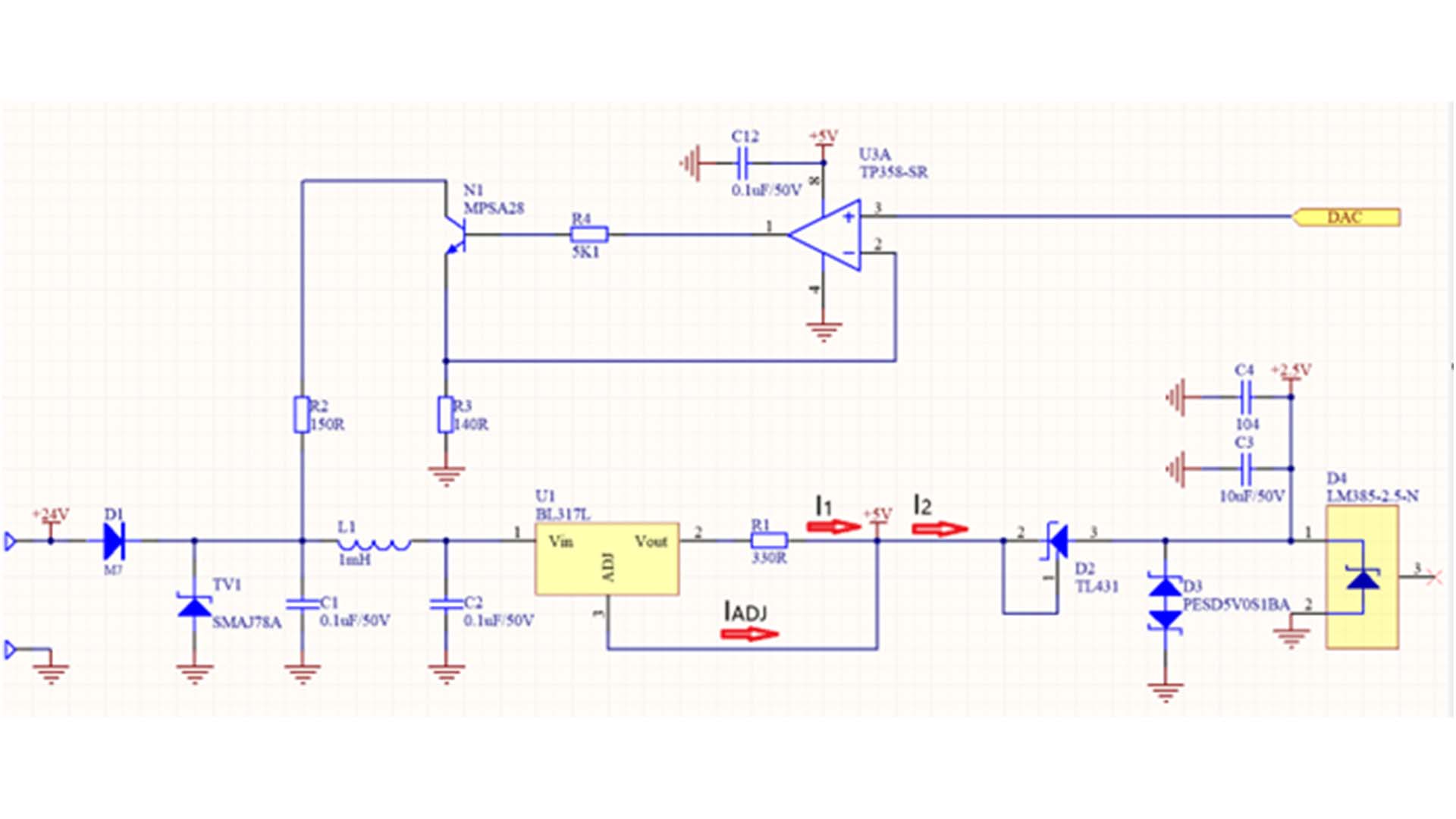
In industrial settings, to save on cabling costs, a 4-20mA two-wire system is commonly used. This system uses two wires to simultaneously power the field sensor/transmitter and transmit the analog signal. We know that the sensor/transmitter circuit requires a certain amount of current to operate; therefore, the circuit structure using this method must be low-power. The 4mA zero-point current ensures that the device can start up and operate normally. The analog signal transmission is achieved by dynamically adjusting a constant current source circuit to ensure that the total current in the loop remains precisely between 4mA and 20mA. Figure 1. Constant current and voltage regulation circuit Figure 2. Internal structure diagram of the LM317 Figure 1 shows a constant current regulator circuit built using the BL317, which is a low-power constant current source circuit that precisely controls the output current to 3.8mA. The circuit ensures that the current flowing into U1 remains constant at 3.8mA, preventing the current from fluctuating with changes in the downstream load. As shown in the internal structure diagram of the LM317 in Figure 2, the voltage between Vout and ADJ remains stable at approximately 1.25V during normal operation, thus the current I1 through resistor R1 also remains constant. The current direction is indicated by arrows, from which the following relationship can be derived: I2 = I1 + IADJ, where IADJ is 50μA and can be neglected. Therefore, I2 is approximately equal to I1, i.e., I2 ≈ I1 = 1.25V/330Ω = 3.8mA. The subsequent stage of the circuit in Figure 1 utilizes the low-power voltage reference diode LM385-2.5 to provide a 2.5V regulated power supply for the low-power system. The LM385-2.5 operates within a current range of 20μA to 20mA and features extremely low dynamic impedance and excellent temperature stability. The circuit also cleverly utilizes the characteristics of the TL431 precision voltage reference source by short-circuiting the reference pin 1 and cathode pin 2 of the TL431 and connecting it in series with the circuit. In this configuration, the voltage drop between the anode and cathode of the TL431 is 2.5V, thus ensuring that the output voltage at the constant current source I2 is 5V. This voltage can provide power for the signal conditioning circuit.
Read More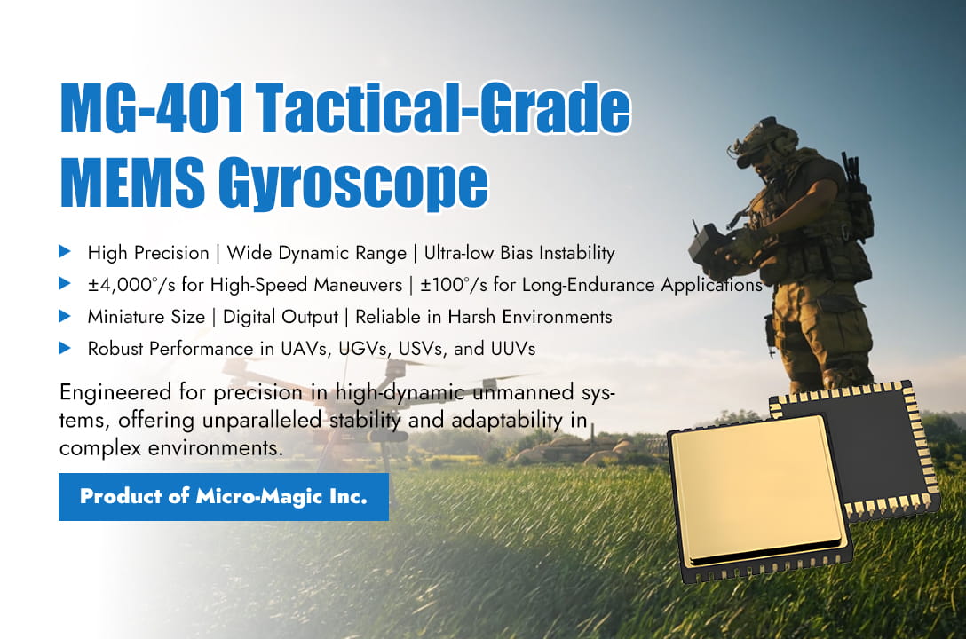
At a pivotal stage in the global advancement of unmanned systems toward intelligence, swarm capabilities, and high precision, the performance of core sensors has become a critical bottleneck limiting system capability enhancement. Recently, Micro-Magic, a leading designer and manufacturer of inertial sensors, officially launched a new generation of tactical-grade single-axis MEMS gyroscope sensor series. This product line, optimized for deep integration with UAVs, UGVs, USVs, UUVs, and various robotic platforms, aims to provide a robust and precise motion sensing foundation for next-generation high-dynamic, highly autonomous unmanned systems, enabling stable operation and intelligent decision-making in complex environments The newly released chip series covers multiple models, including the MG-101/102, MG-401 series, MG-501 series, MG-2001, and MG-4001/4002. Featuring a unified miniaturized ceramic package (10×10×3.5 mm, weighing 1.5 grams) and fully digital output, it delivers a comprehensive solution ranging from ultra-high precision to ultra-wide dynamic range. Its technical specifications directly address the stringent requirements of unmanned systems across diverse scenarios: whether it's the extreme maneuvers of racing drones with up to ±4,000°/s, the stable measurement of minute angular velocities within ±100°/s for underwater submersibles over tens of hours, or the reliable and precise angular rate data provided by the series in rugged terrains against continuous impacts and vibrations for unmanned vehicles. At a pivotal stage in the global advancement of unmanned systems toward intelligence, swarm capabilities, and high precision, the performance of core sensors has become a critical bottleneck limiting system capability enhancement. Recently, Micro-Magic, a leading designer and manufacturer of inertial sensors, officially launched a new generation of tactical-grade single-axis MEMS gyroscope sensor series. This product line, optimized for deep integration with UAVs, UGVs, USVs, UUVs, and various robotic platforms, aims to provide a robust and precise motion sensing foundation for next-generation high-dynamic, highly autonomous unmanned systems, enabling stable operation and intelligent decision-making in complex environments The newly released chip series covers multiple models, including the MG-101/102, MG-401 series, MG-501 series, MG-2001, and MG-4001/4002. Featuring a unified miniaturized ceramic package (10×10×3.5 mm, weighing 1.5 grams) and fully digital output, it delivers a comprehensive solution ranging from ultra-high precision to ultra-wide dynamic range. Its technical specifications directly address the stringent requirements of unmanned systems across diverse scenarios: whether it's the extreme maneuvers of racing drones with up to ±4,000°/s, the stable measurement of minute angular velocities within ±100°/s for underwater submersibles over tens of hours, or the reliable and precise angular rate data provided by the series in rugged terrains against continuous impacts and vibrations for unmanned vehicles. MG401 M-QMG07 M3G-220
Read More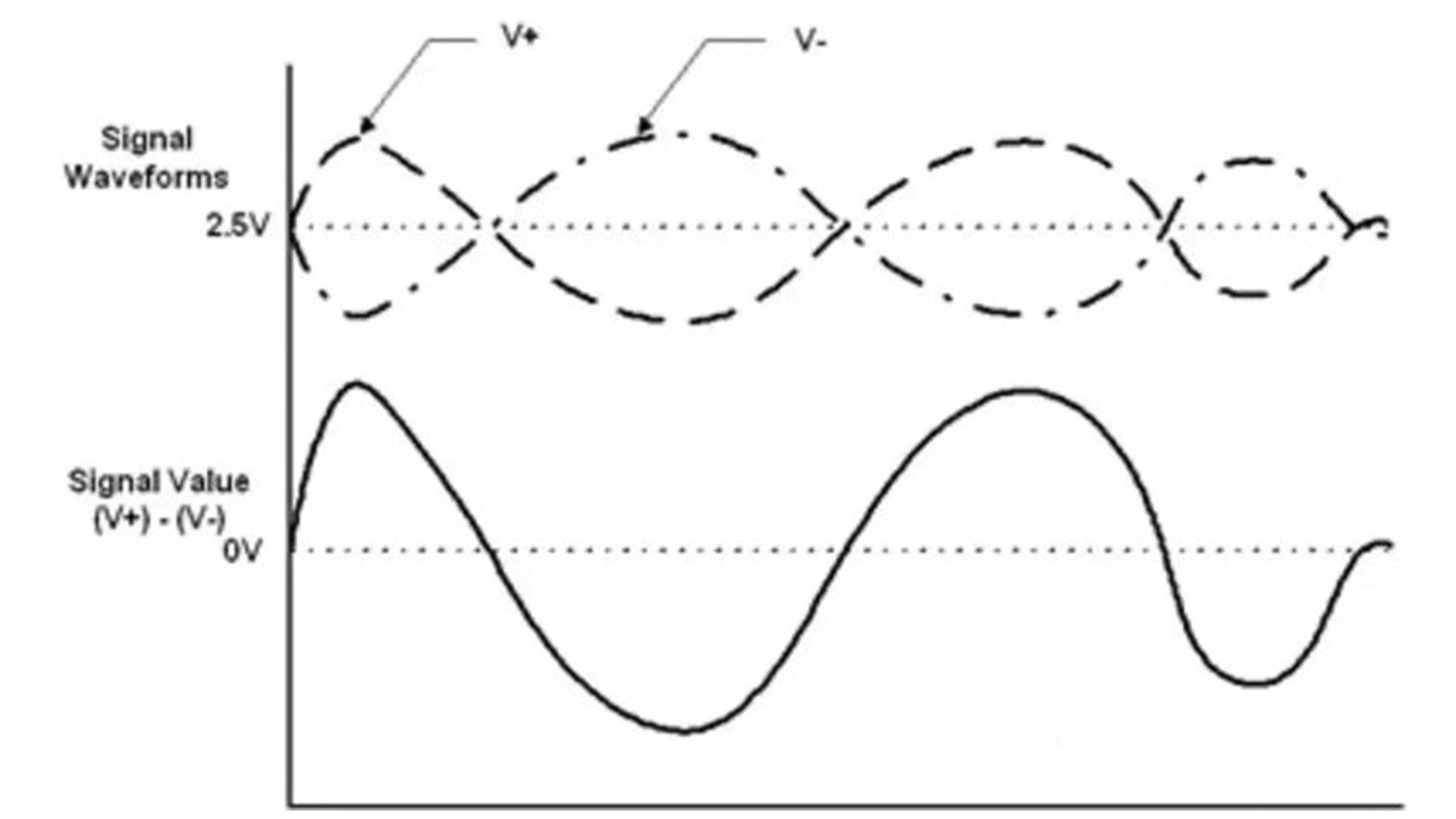
We know that to improve the anti-interference capability of communication systems, RS485, CAN bus, USB, and Ethernet interfaces all use differential signal transmission. Differential transmission is a signal transmission technique that differs from the traditional single-signal-line approach. Differential transmission transmits signals through two lines, with these two signals having equal amplitudes but opposite phases. The signals transmitted on these two lines are called differential signals. A differential signal uses a numerical value to represent the difference between two physical quantities. Differential signals are also called differential-mode signals, as opposed to common-mode signals. Figure 1 shows the transmission waveforms of the V+ and V- differential signals on the signal lines and the data analysis waveforms at the receiving end. Figure 1. Differential signal waveform When we use differential signaling for transmission, although it increases the complexity of any related interface circuits, it offers the following three advantages: 1. Because you are controlling the 'reference' voltage, small signals can be easily identified. In a single-ended signal system using ground as a reference, the accuracy of the measured signal depends on the consistency of the 'ground' within the system. The further the signal source and receiver are from each other, the greater the possibility of differences in their local ground voltage values. The signal value recovered from a differential signal is largely independent of the precise value of the 'ground'; 2. It is highly immune to external electromagnetic interference (EMI). An interference source affects each end of the differential signal pair to almost the same extent. Since the voltage difference determines the signal value, any identical interference appearing on both conductors will be ignored. Besides being less sensitive to interference, differential signals generate less EMI than single-ended signals; 3. In a single-supply system, it can easily and accurately handle 'bipolar' signals. To handle bipolar signals in a single-ended, single-supply system, we must establish a virtual ground at some arbitrary voltage between the ground and the power supply rail (usually the midpoint). Voltages above the virtual ground represent positive signals, and voltages below the virtual ground represent negative signals. Then, the virtual ground must be correctly distributed throughout the system. With differential signaling, such a virtual ground is not needed, allowing us to process and transmit bipolar signals with high fidelity without relying on the stability of the virtual ground.
Read More
In the era of rapid advancement in drone technology, whether for high-definition aerial surveying and mapping, precision agricultural plant protection, or emergency supply delivery and complex environmental monitoring, drones have evolved from simple remote-controlled toys into highly intelligent aerial robots. Behind this transformation lies the flight control system's near-obsessive demand for real-time, precise attitude and motion data. The core technological cornerstone meeting this demand is the micro-electromechanical system (MEMS) inertial sensor—acting as the drone's "inner ear" and "balance nerves," silently sensing every moment of attitude change and motion state. These sensors serve as the physical foundation enabling drones to achieve stable hovering, autonomous navigation, agile maneuvering, and precise control. Traditional high-precision inertial navigation systems rely on bulky, expensive, and power-hungry optical or mechanical gyroscopes and accelerometers, severely limiting their application in consumer-grade and industrial-grade drones that prioritize lightweight, low cost, and long endurance. The groundbreaking advancements in MEMS technology have completely transformed this landscape. By seamlessly integrating micro-scale mechanical sensing structures with integrated circuit processes, it has miniaturized inertial sensors to the chip level. For instance, the ACM-1700 series of high-performance MEMS single-axis accelerometers from Micro-Magic employ advanced MEMS processes, achieving a wide range from ±10g to ±200g, a bandwidth up to 100Hz, and exceptional bias stability (down to 50μg) within a compact package measuring just 7.8 x 5.8 x 3mm. With robust construction capable of withstanding impacts up to 10,000g and full-temperature-range compensation via integrated temperature sensors, the ACM-1700 series ensures reliability and measurement consistency during drone's aggressive maneuvers and in complex environments. Whether monitoring linear acceleration or deceleration of drones or detecting vibrations caused by wind or maneuvers, the ACM-1700 series delivers precise data inputs. ACM-1700 Measuring Range ±10~30/±30~50/±70~100/±150~200g Measuring Axis X Zero Bias Stability (10s, 1σ) 50/100/200/500μg Zero Bias Temperature Coefficient (full temperature) 50/50/100/200μg/℃ Impact Resistance 10000g,2ms,1/2 sine Vibration Rectification Error (6grms) 0.4/0.15/0.05mg Communication Protocol I2C/SPI/UART Output Signal Digital Pack and Size Chip, 7.8*5.8*3mm Weight 1.5g However, perceiving only linear acceleration is insufficient to fully describe a drone's motion state. Rotational motion, specifically angular velocity around three axes, is equally crucial for attitude determination. The MG-XXXX series high-precision MEMS single-axis gyroscope by Micro-Magic is precisely designed for this purpose. This series employs an innovative MEMS structure capable of accurately measuring angular velocity along the rotation axis perpendicular to the chip surface. Its high performance is characterized by extremely low noise and exceptional bias stability, providing precise angular velocity feedback for drone flight control. Through its flexible SPI digital interface and configurable registers (such as adjusting output bandwidth from 12.5Hz to 800Hz or setting data update rates from 62.5Hz to 2000Hz), the flight control system can optimize sensor response for different flight modes (e.g., smooth cruising or agile maneuvers), achieving the best balance between suppressing high-frequency noise and maintaining rapid signal response. The combination of the MG-XX series and the ACM-1700 series forms the fundamental sensing pair for drones to perceive their three-dimensional spatial motion in principle. However, integrating multiple independent, high-performance MEMS sensor chips (three-axis gyroscope + three-axis accelerometer) into drone flight control and processing their raw data to obtain stable and usable attitude information is a complex engineering challenge involving precision calibration, temperature compensation, sensor fusion algorithms, and high-speed data processing. This is precisely where the value of MEMS inertial measurement modules such as U503, U4930, U16575. It is not a simple sensor stack, but a highly integrated and intelligent solution. This type of IMU module is housed in a sturdy aluminum alloy casing and has achieved precise positioning and installation of three-axis MEMS gyroscopes and three-axis MEMS accelerometers, integrating high-performance microprocessors. U503 U4930 U16575 Taking U4930 IMU module as an example, its core progressiveness lies in the full temperature calibration and system level compensation completed before delivery. The processor inside the module not only synchronously collects raw data from six axes at high speed (up to 2000Hz), but more importantly, it applies a pre calibrated compensation parameter matrix over a wide temperature range (-40℃ to +85℃) to perform real-time digital compensation for dozens of error terms such as zero bias error, scale factor nonlinearity, non orthogonal error, and acceleration sensitivity (g-sensitivity) of the gyroscope for each sensor. This allows the module to directly output high-precision angular velocity (°/s) and acceleration (m/s ²) data after temperature calibration and error correction. Users no longer need to perform tedious laboratory level calibration, greatly simplifying system integration and ensuring consistency and reliability of performance under different climate conditions. The RS422 interface it provides can stably output data packets containing angular velocity, acceleration, internal temperature, and high-precision timestamps at a frequency of up to 200Hz. It can also output TOV differential pulse signals that are strictly synchronized with data sampling, facilitating precise time alignment with external systems such as GPS, which is crucial for integrated navigation. In actual drone flight, these clean inertial data from IMU modules are fed in real-time into the core of flight control - attitude calculation and navigation algorithms (usually based on Kalman filters). The algorithm intelligently integrates the specific force information measured by the accelerometer (used to determine the direction of gravity, i.e. pitch and roll angles) with the angular velocity information measured by the gyroscope (used to integrate and obtain attitude changes). Through this' sensor fusion ', the system is able to overcome the respective shortcomings of accelerometers being susceptible to vibration interference during dynamic maneuvers and gyroscope integration drifting over time, thereby outputting stable, accurate, and error free real-time three-dimensional attitude (pitch, roll, yaw), angular velocity, and linear acceleration information. These pieces of information are the foundation of closed-loop control in flight control: the flight control compares the target waypoint or remote control instructions with the current real-time attitude and position, calculates the precise thrust commands of each motor, and drives the drone to complete a series of complex actions such as hovering, climbing, turning, obstacle avoidance, etc. Therefore, from the basic physical quantity perception provided by the chip level ACM-1700 accelerometer and MG-XXXX gyroscope, to the integrated, calibrated, and intelligent data supply achieved by the module level U503, U4930, U16575 inertial measurement units, MEMS inertial sensor technology constitutes a complete technology stack, gradually solving the problem of UAV attitude perception layer by layer. They enable modern drones not only to 'fly', but also to 'fly steadily', 'fly accurately', and 'fly intelligently'. With the improvement of autonomous driving levels and the increase in task complexity, the requirements for the performance of MEMS inertial sensors will also rise. The continuously evolving high-performance and highly integrated MEMS solutions are undoubtedly the indispensable underlying support for future unmanned aerial vehicles to move towards full autonomy, clustering, and intelligence.
Read More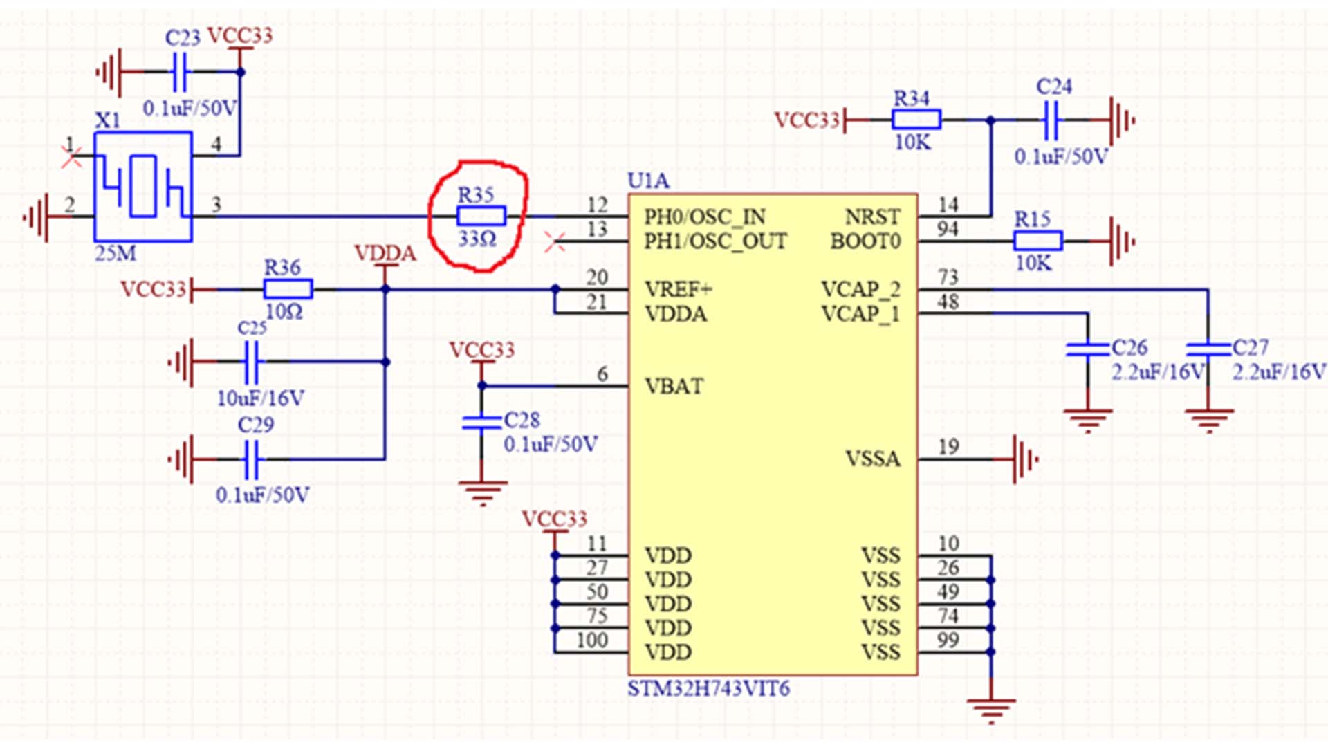
When designing the clock circuit diagram for an MCU, if an active crystal oscillator is used as the clock source, a resistor of several tens of ohms is usually added to its output. This resistor primarily serves the following purposes: 1. Impedance Matching When the output impedance of the active crystal oscillator does not match the impedance of the PCB transmission line (usually 50Ω), it can lead to signal reflection, causing overshoot and ringing. By adding a 33Ω resistor in series at the source (forming a 50Ω match with the crystal oscillator's internal resistance of approximately 20Ω), reflected signals can be absorbed, reducing the reflection coefficient. 2. Reducing EMI The output signal of an active crystal oscillator is a square wave signal. The steep edges and the resulting high-frequency ringing generate a large amount of high-frequency noise, which radiates outwards, leading to electromagnetic compatibility (EMC) problems and potentially affecting other parts of the system or failing EMC testing. The series resistor smooths the signal edges, reducing the high-frequency components of the signal, thus effectively reducing electromagnetic radiation (EMI). This is a low-cost and effective EMI suppression measure. 3. Limiting Crystal Oscillator Output Current and Protecting the Output Stage The output driver inside an active crystal oscillator usually has limited capacity. If the input capacitance of the subsequent load is large, or if an accidental short circuit occurs (although rare), a large instantaneous charging and discharging current will be generated at the moment of the square wave transition (charging current i = C * dv/dt). The series resistor can limit this peak current, reducing the burden on the crystal oscillator's internal output stage, providing a certain degree of protection and improving system reliability.
Read More
On the vast North China Plain, a large agricultural drone with a wingspan of over three meters glides steadily across wheat fields at an altitude of five meters. Unlike traditional spraying operations, this drone maintains exceptional stability while navigating undulating field ridges and fluctuating air currents, delivering uniformly atomized pesticide mist with clear, non-overlapping boundaries. The core behind this precise operation is its "Flight Central Unit"—the U16575 MEMS high-precision inertial measurement unit (IMU) recently introduced by Micro-Magic Inc. This sensor, hailed as the "industrial-grade intelligent perception core," is providing reliable technological support for the application of large drones in fields such as precision agriculture, thanks to its exceptional stability and accuracy. The terrain and climate challenges faced by large agricultural drones far exceed those of consumer grade models. The low altitude airflow disorder in the fields, the continuous high-frequency vibration caused by the engine and rotor, and the rigorous test of sensor stability for several hours of cross temperature operation are all major challenges that must be overcome to achieve technological upgrades such as uniform spraying and variable fertilization. The launch of high-precision IMU U16575 directly addresses these pain points. It integrates high-performance three-axis MEMS gyroscopes and three-axis MEMS accelerometers internally, and uses a system level compensation algorithm in the full temperature range (-40°C to +80°C) to real-time correct zero bias, scale factor, and even non orthogonal errors between axes, ensuring that attitude perception data is always accurate and consistent during all-weather operations of the drone from low morning temperatures to high afternoon temperatures. Stability is the cornerstone of agricultural efficiency, "said the technical expert from Micro-Magic. U16575 performs excellently in terms of parameters: gyroscope zero bias instability ≤1°/h, angle random walk ≤0.2°/√h; accelerometer zero bias instability ≤ 30μg. This means that even when the drone is turning or encountering gusts of wind, the IMU can provide extremely small noise and drift data, allowing the flight control system to quickly build high-precision attitude closed-loop control, thereby firmly locking in the preset flight altitude and route. For drones that need to use terrain following functions to operate on terraced fields or slopes, this' stability 'is crucial. In addition to accuracy, reliability is another lifeline for the large drone industry. U16575 adopts a lightweight aluminum alloy structure, which combines high strength with excellent vibration resistance and shock resistance, and can easily cope with the harsh mechanical environment of drone takeoff and landing and operation. Its compact size (22.4*22.3*13.7mm) and lightweight weight (about 12g) also contribute to the valuable payload space and endurance of the drone. "We have observed that an increasing number of drone system integrators require not only high performance but also complete solutions with 'high usability' and 'high reliability'," stated the sales director of Micro-Magic. "The hardware compatibility between the U16575 and the ADIS16575, coupled with the comprehensive technical support and communication protocols we provide, enables customers to swiftly complete product upgrades and verification, thereby shortening the time-to-market cycle." From precise spraying to surveying and exploration, from power inspection to logistics transportation, as the application scenarios of large-scale drones continue to deepen, the requirements for their "perception nerves" are becoming increasingly stringent. The U16575 high-precision IMU, with industrial grade performance, military grade reliability, and commercial grade cost, is becoming an indispensable key component in the high-end unmanned aerial vehicle field, helping unmanned systems achieve more accurate, reliable, and intelligent flight in a wider world.
Read More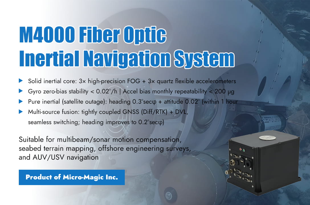
The core challenge in marine surveying lies in accurately determining the position, attitude, and motion state of the survey platform in open ocean environments where stable external references are lacking, thereby providing a stable spatial reference for detection equipment such as sonar. Traditional GPS+gyrocompass solutions can function under calm sea conditions, however, once encountering rough seas, the rolling, pitching, and heaving movements of the vessel can severely interfere with measurement accuracy, not to mention in complex submarine canyons or areas with electromagnetic interference, where GPS signal interruptions can bring the entire survey mission to a standstill. The M4000 Fiber Optic Inertial Navigation System, developed by Micro-Magic Inc, was specifically designed to address this critical pain point. The outstanding performance of the M4000 system begins with its solid fiber optic inertial core. The system integrates three high-precision fiber optic gyroscopes and three quartz flexible accelerometers internally, forming a stable and reliable autonomous sensing foundation with gyroscope's zero bias stability better than 0.02 °/h and accelerometer's bias monthly repeatability less than 200ug. This foundation enables the system to maintain a heading accuracy of 0.3°secφ and an attitude accuracy of 0.02° within 1 hour even in pure inertial mode with satellite signal interruption, providing a continuous and uninterrupted attitude reference for surveying operations and ensuring the spatiotemporal continuity of data acquisition. The true technological breakthrough is reflected in its powerful multi-source information fusion capability. The M4000 is not simply a stack of sensors, but a smart integrated navigation system with fiber optic inertia as the core, deeply coupled with GNSS satellite navigation and DVL Doppler odometer. When the satellite guidance signal is good, the system tightly combines with built-in or externally connected GPS (supporting differential and even RTK) to effectively correct accumulated inertial errors, improve heading accuracy to 0.2°secφ, and provide high-precision real-time position and velocity information. More importantly, in the face of the challenge of satellite navigation signal loss caused by underwater, fjord or complex sea conditions, the system can seamlessly integrate DVL, continuously suppress navigation error divergence using bottom or water velocity information, and ensure uninterrupted navigation solutions and accuracy during critical tasks. The ability to intelligently adapt and smoothly switch between "satellite navigation combination" and "pure inertia" modes gives surveying vessels or underwater vehicles the freedom to operate in all weather and sea conditions. In response to the precise perception requirements of vertical motion in marine surveying, the M4000 has specifically optimized its heave measurement function, with an accuracy of up to 5 centimeters or 5% heave amplitude. It can effectively separate the ship's own motion from wave disturbances, providing crucial motion compensation for multi beam depth measurement data and directly improving the quality of seabed terrain models. At the same time, the system takes into account the convenience and stability of engineering applications. Built in 32GB storage card can record complete navigation data for a long time and remotely read it through the network; Rich configurable interfaces and multi-channel synchronous pulse outputs enable it to flexibly connect to various surveying sensors and ensure data spatiotemporal synchronization. Its embedded IE configuration interface makes device control and parameter binding (such as installation deviation and lever arm compensation) more intuitive and convenient, greatly reducing the technical threshold for system integration and maintenance. From extensive terrain scanning in vast sea areas to precise underwater engineering investigations, and from precise positioning of surface surveying ships to reliable navigation of autonomous underwater vehicles, The M4000 fiber optic inertial navigation system, with its high-performance inertial core, deep fusion integrated navigation strategy, and highly engineered design, is becoming a key enabler for improving the quality and operational efficiency of marine surveying data. It not only represents the advancement of precision instruments, but also signifies the powerful ability to provide all-weather, highly reliable, and integrated solutions in the field of high-end ocean navigation and positioning, laying a solid technological foundation for managing the ocean and expanding blue territories.
Read More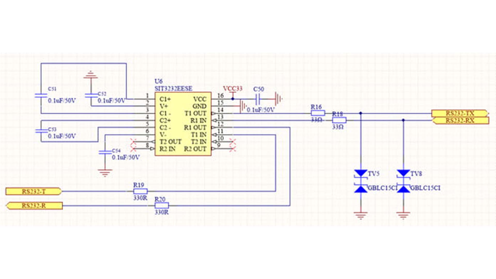
The function of a TVS (Transient Voltage Suppressor) is to protect electronic circuits from damage caused by transient overvoltages (such as lightning strikes and electrostatic discharge). It ensures circuit safety by rapidly clamping and diverting surge energy. In TVS protection circuit design, a resistor is usually connected in series, as shown in Figure 1, where a 22Ω resistor is connected in series with both the receiving and transmitting lines of the RS232 communication interface circuit. The TVS is connected in series with the resistor to absorb energy during overvoltage events, protecting the circuit and limiting the current. This configuration ensures that when the circuit is threatened by transient overvoltage, the TVS can quickly intervene and effectively absorb the overvoltage, thus protecting other components in the circuit from damage. At the same time, the series resistor further regulates the current magnitude, preventing the TVS from being damaged by excessive current while absorbing the overvoltage. Figure 1 RS232 communication interface There are generally two ways to connect a TVS with a series resistor: one is to place the resistor after the TVS, as shown in Figure 2, and the other is to connect the resistor before the TVS, as shown in Figure 3. These two methods vary depending on the application scenario. The front connection method can reduce inrush current, while the rear connection method can more effectively perform secondary voltage division and current limiting. Figure 2 Figure 3 In the circuit shown in Figure 2, the TVS device initially absorbs most of the inrush current. Subsequently, any remaining residual voltage or current is divided and current-limited again through resistor R2. This design more effectively protects the downstream load. However, if the impedance of the downstream load is much greater than that of resistor R2, the voltage division and current-limiting effect becomes relatively small, and the role of resistor R2 is relatively weakened. In the circuit shown in Figure 3, when considering the magnitude of the inrush current, if the surge is small, a resistor of appropriate power can be selected and placed before the TVS. In this way, the resistor will share a small portion of the current, thereby reducing the inrush current IPP. Consequently, the clamping voltage Vc of the TVS will also decrease accordingly, further enhancing the protection effect on the downstream load.
Read More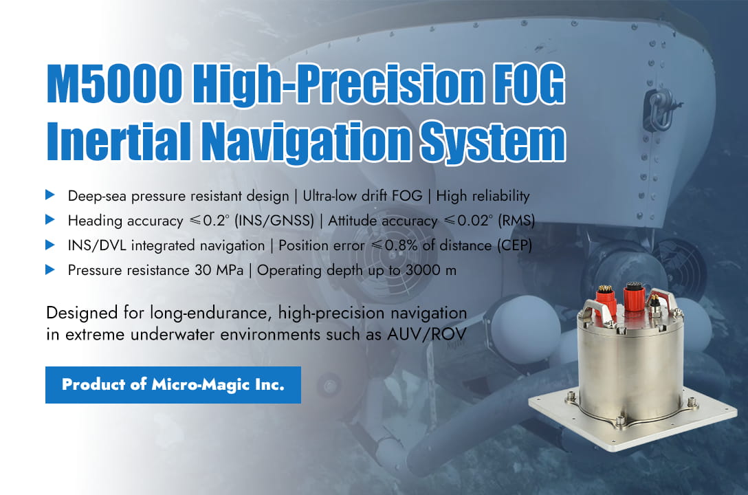
Deep sea exploration faces severe challenges such as high pressure, darkness, complex electromagnetic environments, and long endurance operations. In equipment such as unmanned deep-sea submersibles and underwater mapping platforms, high-precision and high reliability inertial navigation systems (INS) are the core to ensure the success of missions and the key technology to achieve autonomous, precise, and long-term underwater operations. Taking the M5000 pressure resistant fiber optic gyroscope (FOG) strapdown inertial navigation system produced by Micro Magic as an example, it has become the core navigation solution for deep-sea vehicles (such as AUV/ROV) with its deep-water pressure resistant design, multi-source fusion navigation capability, and high-precision sensors. Long-Endurance AUV Autonomous Exploration and Mapping AUVs need to conduct autonomous navigation for several hours or even days in thousands of meters deep trenches without GPS signals and with complex terrain, to perform large-scale underwater terrain mapping, resource surveys, or environmental monitoring. The system must have the ability to achieve long-term high-precision positioning, stable attitude output, and effectively integrate DVL velocity information to suppress accumulated errors in inertial navigation. The M5000 inertial navigation system integrates ultra-low drift FOG (0.01°/h) and high-precision accelerometer (0.02m/s²), ensuring extremely high attitude and heading accuracy during long-term underwater navigation, providing a stable platform and accurate geographic reference for surveying sensors (multi beam, side scan sonar). At the same time, the M5000 deeply integrated INS/DVL, significantly improving underwater positioning accuracy. A circular probability error of 0.8% of the range means that after sailing 10 kilometers, the positioning error is only about 80 meters (CEP), which is much better than pure inertial navigation. At a depth of 3000 meters and a pressure resistance of 30 MPa, it directly meets the depth requirements of most deep-sea AUV operations without the need for additional pressure tank protection. It is equipped with a 32GB SD card that can fully record the original inertial data and navigation solution results of the entire navigation process, making it easy to replay and analyze, evaluate accuracy, and optimize algorithms after the mission. ROV Precision Tasks and Station Keeping ROV perform precise operations such as equipment deployment, sample collection, and structural maintenance on the seabed, requiring ultra-high instantaneous attitude measurement accuracy and stability to ensure accurate spatial positioning of robotic arm operations; At the same time, it is necessary to quickly respond to the movement of the mother ship and maintain stable hovering. The M5000 provides near real-time precise spatial reference for ROV platforms and robotic arms with ultra-high attitude accuracy (≤0.02° RMS), which is the key to successful precision operations; 5cm or 5% surge accuracy, effectively measuring the vertical (heave) motion caused by the mother ship or ocean current, combined with high-precision attitude, assisting the ROV stability control system to achieve precise hovering and anti surge interference. Seafloor Observatories and Landers Observation platforms or landers that are deployed on the seabed for a long time need to monitor their own small posture changes (such as seabed geological activity, tilt caused by ocean currents), or provide accurate navigation information during deployment/retrieval. The M5000 inertial navigation system, with ultra-high attitude accuracy and stability, can sensitively capture small attitude changes of the platform, providing important data for geophysical or environmental monitoring; At the same time, M5000, with its independently developed anti electromagnetic interference algorithm, has strong anti-interference ability, which is particularly important in deep-sea hydrothermal areas or equipment intensive platforms where strong magnetic fields may exist; Built in GNSS receiver, quickly obtains accurate position information before deployment (on the water surface) or after recovery, and provides support for dynamic alignment. M5000 Performance Parameter Indicators Parameter M5000 Heading accuracy Inertial/satellite combination: ≤ 0.2° * sec (L) (RMS) Pure inertia: ≤ 0.3 ° * sec (L) (RMS) Attitude accuracy ≤0.02°(RMS) Positioning accuracy ≤0.8%D(CEP,INS/DVL组合) Heave accuracy 5cm or 5%H (Take the maximum value) Angular velocity accuracy 0.01°/s Angular velocity range ±500°/s Acceleration accuracy 0.02m/s^2 Acceleration range ±15g Alignment time ≤5min(Self-alignment) Navigation mode Inertial/satellite combination, pure inertia Operation temperature -40℃~+60℃ Protection grade Pressure resistance of 30 megapascals (3000 meters underwater) Conclusion The M5000 FOG strapdown inertial navigation system, with its deep-sea level pressure resistance capability, FOG based high precision and stability, depth optimized INS/DVL integrated navigation performance, compact and robust design, and rich functions for deep-sea applications, provides powerful navigation, positioning, and attitude reference support for key application scenarios such as autonomous exploration of deep-sea AUV, ROV precision operations, and underwater observation platforms. It is not only the "eyes" of the submersible to perceive its own state and position in a dark and high-pressure environment, but also the "nerve center" to ensure accurate and reliable detection data and successful execution of operational tasks.
Read More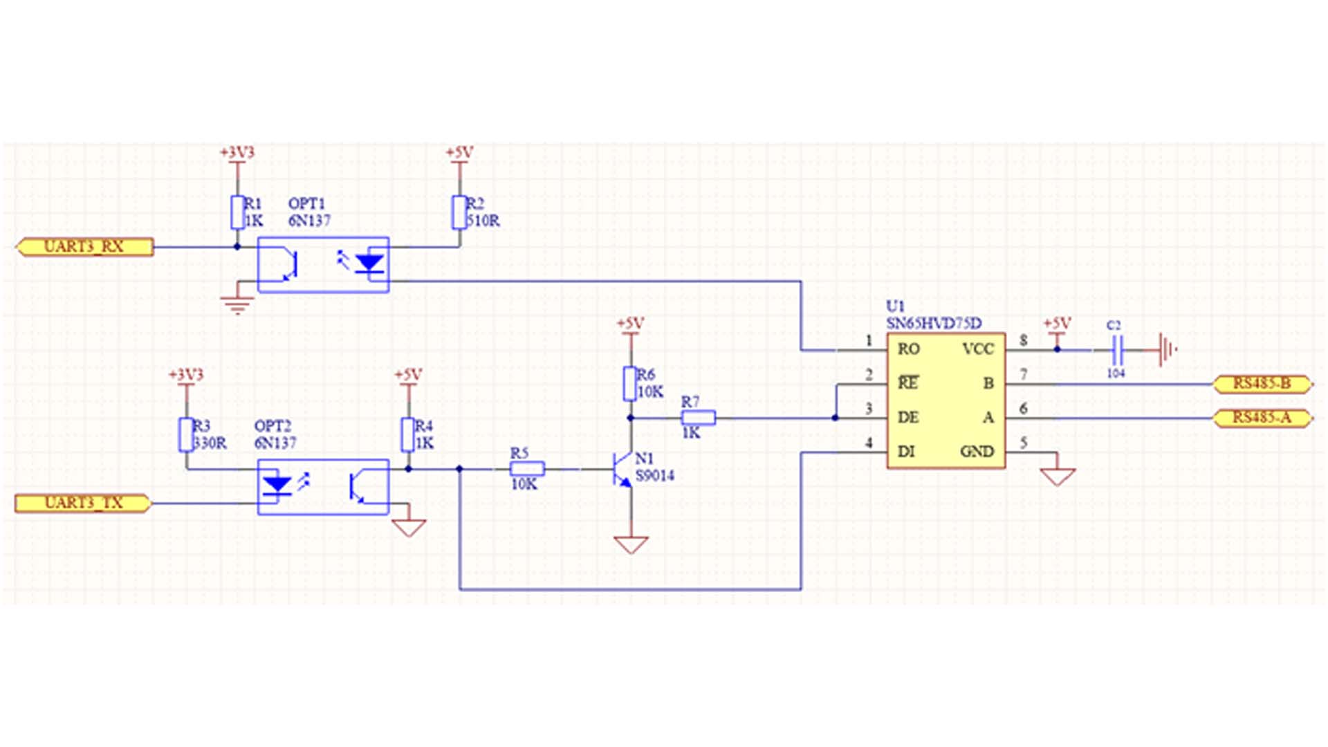
RS485 is widely used in various fields such as industrial intelligent instruments and communication equipment due to its strong anti-interference ability and low cost. However, industrial environments are complex and subject to severe electromagnetic interference. Non-isolated RS485 systems have the following disadvantages: (1) In outdoor or industrial environments, lightning strikes and power switching can generate transient high-voltage surges, which can easily damage the backend circuit; (2) When multiple devices share the RS485 bus, a fault at one node (such as a short circuit) can cause the entire bus to fail; (3) When the distance between 485 communication nodes is too far (greater than 50 meters), the reference ground of each node is connected to the local ground. When there is a large voltage difference between the grounds at both ends, the ground potential will be superimposed on the signal line as a common-mode voltage, which may exceed the common-mode voltage range that the port can withstand, affecting normal communication, or even damaging the backend circuit; (4) When the ground planes between distant 485 communication nodes are connected using cables (such as 485 shielded cables), the ground wire will form a ground loop with the earth, coupling external common-mode noise and generating ground loop currents, which may cause the entire circuit system to fail. If these unfavorable factors exist, or if safety regulations require electrical isolation between devices to prevent leakage or sparks from causing hazards, an isolated RS485 solution must be considered. An isolated RS485 circuit adds electrical isolation capabilities to the non-isolated circuit, resulting in stronger anti-interference and system stability. Achieving isolation in an RS485 circuit requires the use of isolation devices, such as optocouplers, magnetic isolators, and isolation chips. Optocouplers are the most commonly used isolation devices and are relatively inexpensive. The speed of the optocoupler must meet the baud rate requirements; generally, high-speed optocouplers are used for RS485 electrical isolation, and a DC-DC isolation module is needed to provide independent power to the node. Figure 1 shows a low-cost RS485 electrical isolation solution.
Read More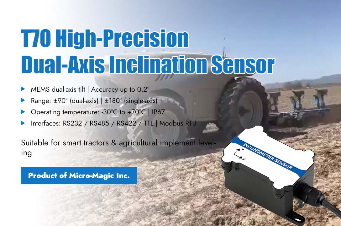
With the acceleration of agricultural modernization, intelligent agricultural machinery has become a crucial equipment for enhancing operational efficiency and ensuring operational safety. Recently, the T70 series high-precision dual-axis inclination sensor launched by Micro-Magic Inc has been successfully applied by customers for real-time monitoring and intelligent control of agricultural machinery posture, providing precise posture feedback for tasks such as sowing, fertilizing, and harvesting. The application of this sensor has significantly improved the consistency and precision of operations, facilitating more scientific and precise agricultural management. At the same time, it also provides reliable data support for the automation upgrade of agricultural machinery, further promoting the development of agricultural production towards intelligence and efficiency. The T70 series tilt sensor utilizes MEMS technology, featuring dual-axis inclination measurement capability with an accuracy of up to 0.2°. It supports a wide range of measurement options, including ±90° (dual-axis) and ±180° (single-axis). Its wide operating temperature range (-30°C to +70°C) and IP67 protection level ensure stable operation even in complex field environments. The sensor supports multiple output modes such as RS232, RS485, RS422, and TTL, and incorporates the Modbus RTU protocol, facilitating integration into various agricultural machinery control systems. In the customer's intelligent tractor project, the T70 inclination sensor is integrated into the latest generation of the tractor suspension system to monitor the horizontal and vertical inclination angles of agricultural machinery in real time. During actual operations, especially on sloping fields and uneven plots, agricultural machinery is prone to operational efficiency decline or even safety accidents due to imbalance in posture. By installing the T70 sensor at key positions on the suspension frame, the system can acquire the inclination data of the machinery in real time and automatically adjust the hydraulic suspension through the controller to achieve dynamic leveling. This not only improves the consistency and quality of operations such as sowing, fertilizing, and harvesting, but also significantly reduces operational difficulty and driver fatigue. The technical leader of the enterprise stated, "The high precision and strong anti-interference capability of the T70 series sensors make them highly suitable for agricultural environments with significant vibrations and drastic changes in temperature and humidity. Their dual-axis synchronous output function allows us to simultaneously monitor the attitude changes in both the forward and backward directions, as well as the left and right directions, enabling true three-dimensional attitude control." In addition, the sensor supports a "relative zero point" setting function, facilitating rapid calibration before operation; the automatic output rate can reach up to 50Hz, meeting the real-time response requirements for high-speed operations. These features collectively support a highly reliable and easily integratable intelligent attitude control system for agricultural machinery. As a leading designer and manufacturer of inertial sensors in China, Micro-Magic is committed to providing high-performance and high-reliability sensor solutions for various industrial and agricultural equipment. The successful application of the T70 series inclination sensors once again demonstrates the company's firm commitment to continuously empowering the upgrading of intelligent equipment through core inertial technology.
Read More
RS232 (also known as EIA RS-232) is one of the commonly used serial communication interface standards. It uses full-duplex communication and requires three lines: ground, transmit, and receive. RS-232 is only suitable for point-to-point communication between devices. Due to its single-ended signal, it has poor anti-interference capabilities. Therefore, RS232 improves signal anti-interference and increases transmission distance by increasing the voltage level. RS232 uses negative logic levels, with a logic 0 level of [3, 15]V and a logic 1 level of [-15, -3]V. The maximum transmission distance of the RS232 standard is affected by many factors, mainly depending on the transmission rate, cable characteristics, chip driving capability, and signal transmission characteristics. 1. Transmission Rate Transmission distance is inversely proportional to the baud rate. The higher the baud rate, the more severe the signal attenuation and distortion. At 19.2 kbps, the distance usually does not exceed 15 meters. At 9.6 kbps, the distance can reach 30-50 meters. At rates as low as 1.2 kbps, it may reach 300 meters (with other conditions optimized). 2. Cable Characteristics The RS232C standard specifies that the driver is allowed to have a capacitive load of 2500 picofarads. When using a communication cable with a capacitance of 150 picofarads per meter, the maximum communication distance can reach 15 meters. If the capacitance per meter of the cable is reduced, the communication distance can theoretically be increased accordingly. 3. Chip Driving Capability Early chips had weaker driving capabilities, while modern chips (such as MAX232) can support longer distances with driving currents reaching 1mA. 4. Signal Transmission Characteristics • RS232 uses a single-ended signal transmission method, which has problems such as common-ground noise and the inability to effectively suppress common-mode interference, further limiting its transmission distance. Using shielded cables to reduce external electromagnetic interference can also increase the transmission distance. In practical applications, RS232 communication lines are usually used for short-distance communication within 20 meters.
Read Moreleave a message
Scan to Wechat :