Applications

The 3D electronic compass is the core sensor component for achieving spatial orientation and attitude perception in modern AR/VR systems, and its technology is based on multi-sensor fusion for complex systems. This device can measure the absolute direction of the equipment in three-dimensional space in real time by integrating three-axis flux gate sensors, three-axis MEMS accelerometers, and/or three-axis gyroscopes. The flux gate sensor is responsible for detecting the components of the Earth's magnetic field vector on three orthogonal axes, the accelerometer senses the direction of gravity to determine pitch and roll angles, and the gyroscope provides angular velocity information for dynamic attitude compensation. This multi-sensor architecture enables electronic compasses to maintain heading accuracy in complex motion states, providing a stable directional reference for AR/VR applications. Key Technical Characteristics and Performance Parameters The performance of a 3D electronic compass directly affects the user experience of AR/VR systems. Modern devices such as C9000 series high-precision 3D electronic compass can maintain heading accuracy at extreme tilt angles of ±85°, which is achieved through three-axis accelerometers for heading compensation of a wide range of tilt angles. This anti tilt ability is particularly important for AR headsets and VR controllers, as users often experience significant head or hand movements during use. In addition, high-performance electronic compasses also use hard/soft iron calibration technology to reduce environmental interference and ensure measurement stability in metal environments. Parameter C90 C9000 The impact on AR/VR Heading range 0~360° 0~360° Full range tracking Heading accuracy 0.3~0.5° 0.2° Affects the alignment accuracy of virtual objects Tilt Angle Range Pitch ±90°;  Roll 360° Pitch ±90°; Roll 360° Support large angle head rotation Tilt Angle accuracy 0.1° 0.02° Insufficient accuracy can lead to virtual object drift, screen shaking Response time 20ms 20ms Reduce virtual object latency Calibration Hard magnetic, soft magnetic, and tilt compensation Hard magnetic, soft magnetic, and tilt compensation Ensure stable and accurate orientation of virtual objects, enhance immersion, and avoid dizziness. Product Form Module/ Single-Board Module/ Single-Board Easy for secondary integration development or embedding within devices       Application of 3D Electronic Compass in AR Navigation and Outdoor Exploration   Virtual real registration is the core challenge of AR navigation, requiring seamless overlay of virtual navigation indicators to the correct position in the real scene. By using the azimuth, elevation, and roll angles provided by the 3D electronic compass, the system calculates the rotation matrix and translation vector of the camera coordinate system relative to the world coordinate system, and constructs a transformation matrix from the world coordinate system to the camera coordinate system, providing users with intuitive directional guidance. When the user turns on AR mode, the system captures the surrounding environment through the camera, and at the same time calls the direction data of the electronic compass and the position data of GPS to generate 3D navigation arrows that are integrated with the environment. The system can also support offline map function, relying on electronic compass and inertial navigation to continue providing directional guidance in remote areas without network signals, greatly expanding the applicability of AR navigation.     Application of 3D Electronic Compass in Indoor AR Navigation and Equipment Display The indoor environment poses a serious challenge to traditional positioning technology due to the lack of GPS signals and the presence of complex magnetic interference sources. A high-precision indoor AR navigation system was constructed by combining a 3D electronic compass with IR-UWB ultra wideband positioning and image moment feature recognition. This innovative solution is the first to apply IR-UWB technology to 3D registration in augmented reality, achieving centimeter level positioning accuracy. The system consists of multiple technical modules: CMOS cameras capture real scenes; Helmet mounted displays display enhanced content; The IR-UWB module provides precise position tracking; Three dimensional electronic compass measures the viewing angle direction; Image moment feature module for identifying exhibits; Virtual scene generation module creates virtual content; The virtual real fusion module seamlessly integrates virtual content with real scenes.     Application of 3D Electronic Compass in Immersive VR Experience and Virtual Gimbal   The 3D electronic compass has demonstrated unique value in the field of virtual reality, especially in immersive experiences that require real directional mapping. By introducing real-world directional benchmarks into virtual environments, the electronic compass solves the problem of inconsistent direction perception in VR systems, significantly reducing users' dizziness and tendency to lose direction. In high-end VR systems, a 3D electronic compass is integrated with MEMS sensors to construct an omnidirectional tracking reference, enabling the virtual camera to accurately reproduce the true rotation angle and direction of the user's head. The virtual gimbal based on electronic compass and MEMS system represents the technological innovation of VR interactive devices. This system does not require heavy mechanical structures. It measures three-dimensional geomagnetic field data through an electronic compass, and combines MEMS accelerometer and gyroscope data to calculate the relative azimuth and attitude angle of the gimbal, as well as the zoom and focus information of the camera lens.     Conclusion   The core value of electronic compass in AR/VR lies in providing reliable directional reference and spatial context, and its technological evolution is driving devices to upgrade from "visual immersion" to "multi sensory collaborative interaction". With the continuous emergence of new materials, algorithms, and sensors, the role of electronic compasses in AR/VR systems will become even more important, ultimately achieving the ultimate goal of seamless integration of virtual and real worlds. C9-B C90-C C9000-A C9000-B

LDOs regulate their output voltage to ensure stable operation under varying load current demands. However, when the load current exceeds the designed range, such as in a short circuit or overload, the excessive current can cause chip overheating or even damage. To address this, overcurrent protection mechanisms have emerged to limit the output current and protect both the LDO and its load. LDOs typically have two overcurrent protection mechanisms: brick-wall current limiting and overcurrent shutdown. 1. Brick-Wall Current Limiting   As the name suggests, brick-wall current limiting is a "hard" cutoff mechanism. When the output current exceeds the preset current limit, I_LIMIT,   the LDO quickly limits the output current to I_LIMIT. Due to the high load current, the LDO temperature gradually rises. Once the LDO protection temperature is triggered, the LDO output is immediately shut down. The output voltage-current curve resembles a "brick wall" preventing further current increase. For example, the TPS7A16 data sheet lists its brick-wall current limit threshold at 105mA (typical). As can be seen from the output voltage-load current curve in the figure above, when the load current exceeds I_LIMIT and triggers the LDO temperature protection, the output voltage drops sharply. This mechanism is typically implemented through an internal current sensing circuit combined with a temperature protection circuit. The LDO's internal structure includes a current mirror to detect current. When the sensed current exceeds the set reference current, the current limit is triggered, the LDO temperature rises, and when it reaches the protection temperature, the power transistor is turned off, cutting off the output. This indicates that brick-wall current limiting is safer during short-term overloads. Its characteristic is that it can tolerate short-term overloads, but if the overload persists, heat accumulation will trigger thermal shutdown. 2. Foldback Current Limit Foldback current limiting is very similar to standard upper-limit limiting. However, its primary purpose is to limit total power dissipation. This means that as VOUT decreases and VIN remains stable, the output current limit is linearly reduced to keep the output transistor within a safe power dissipation limit. Devices such as the TLV717P incorporate and benefit from foldback current limiting because they are primarily housed in ultra-small packages with higher thermal resistance. The output current limit behavior of the TLV717P is shown in Figure 3. As can be seen, since VIN is specified at VOUT + 0.5V, the maximum allowable power dissipation at 25°C is 150mW. After the current limit is exceeded and VOUT begins to decrease (assuming RLOAD is constant), both IOUT and power dissipation decrease. This adds a slight complexity to non-ohmic devices that consume a constant current and can trigger a latched state where the powered device continues to reduce VOUT and the LDO continues to reduce IOUT. 3. Overcurrent Shutdown Unlike brick-wall current limiting and foldback current limiting, overcurrent shutdown protection utilizes a fast internal shutdown mechanism. The LDO's internal structure incorporates a current mirror to sense current and a comparator to achieve rapid overcurrent output shutdown. When the LDO output current reaches the overcurrent protection level, the LDO shuts down immediately. Therefore, current threshold protection is faster than brick-wall current limiting and foldback current limiting. If the LDO output is loaded with a large capacitive load, the LDO output will experience a large inrush current, potentially triggering the LDO's overcurrent shutdown mechanism and preventing it from starting properly. In this situation, an LDO with overcurrent shutdown should not be selected.

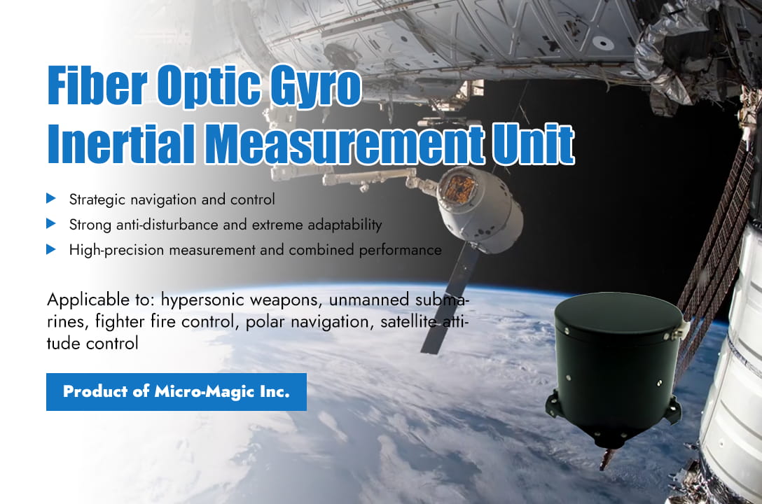
Quickly browse the article in one minute Fiber optic gyroscope IMU (FOG IMU) and MEMS IMU have significant differences in accuracy, environmental adaptability, reliability, and other aspects due to differences in technical principles. The position of fiber optic gyroscope IMU is still irreplaceable in the fields of strategic weapons, deep space/deep-sea exploration, high dynamic military systems, and scientific instruments. Its core advantages lie in the physical limit level accuracy, full temperature stability, and extreme environmental resistance. Even if some high-end MEMS approach tactical level performance, they still cannot meet the strategic level requirements of cutting-edge defense technology.   Core applications in the field of cutting-edge defense technology   1.       Strategic level military equipment navigation and guidance   Intercontinental ballistic missiles and strategic nuclear submarines need to maintain ultra-high precision positioning (zero bias stability ≤ 0.05 °/h) in environments without satellite signals (such as deep sea or space), and resist strong impacts (>25g), extreme temperatures (-45℃~70℃), and electromagnetic interference. The zero bias stability (usually ≥ 0.1°/h) and shock resistance of MEMS IMU are insufficient, and error accumulation can lead to guidance deviation from the target. In satellite attitude control, the space environment requires microradian level angular velocity measurement (random walk ≤ 0.005°/√ h) and long-term stability (MTBF>20000 hours). The thermal stability and radiation resistance of fiber optic gyroscopes are superior to MEMS, which performs better in vacuum and Drift easily under radiation.   2.       Strong electromagnetic interference and high dynamic tactical systems   In the strong electromagnetic field of electronic warfare platforms (such as radar jammers), MEMS is prone to data jumps due to the susceptibility of semiconductor structures to interference, while fiber optic gyroscopes adopt an all-optical design and have non-magnetic material characteristics that can completely resist electromagnetic interference. During the guidance process of hypersonic aircraft, severe vibrations and high temperatures are generated during ultra high speed flight (>5 Mach). The IMU composed of fiber optic gyroscope and quartz accelerometer can withstand 100g impact and 2000Hz vibration, while the MEMS structure is prone to resonance failure. In the fire control system of military fighter jets, real-time attitude angle calculation (error<0.01 °) is required during high maneuverability flight (such as 9g overload). The dynamic response linearity of fiber optic gyroscope (scale factor nonlinearity ≤ 50ppm) is much better than MEMS (≥ 500ppm).   3.       Deep sea exploration and autonomous underwater navigation In the application field of unmanned underwater vehicles (AUV/ROV) and underwater seismometers, pure inertial navigation is required for several months in deep sea environments without GPS, and the position error needs to be less than 1% of the navigation distance. The long-term zero bias stability of fiber optic gyroscope (≤ 0.1°/h) and the low noise of quartz accelerometer (≤ 100 μg) can support microgravity measurement, while MEMS temperature drift (≥ 500 μg) and noise accumulation lead to positioning drift. For example, in underwater pipeline inspection, if the cumulative error exceeds 10 meters, it may cause equipment damage.   4.       Scientific exploration and precision surveying   In gravity gradient measurement and polar scientific exploration, polar magnetic field interference is large and there is no geomagnetic reference. The non-magnetic characteristics of fiber optic gyroscopes can achieve autonomous north finding (heading accuracy ≤ 0.08 °), while MEMS relies on magnetometers and fails in polar regions.   In the deep space orbit calibration of spacecraft, relying on the combination of starlight and inertia navigation, the angle random walk of fiber optic gyroscope (≤ 0.002°/√h) approaches the quantum limit, and the MEMS noise is one to two orders of magnitude higher (≥ 0.03 °/√ h) Key performance comparison   The following table summarizes the irreplaceable core advantages of FOG IMU:  Performance Index FOG IMU MEMS IMU Impact scenario Zero bias stability ≤ 0.05°/h (Strategic level) ≥ 0.1°/h (Tactical level) Long term lack of satellite navigation accuracy angle random walk ≤ 0.002°/√h ≥ 0.03°/√h High precision attitude control anti-electromagnetic interference All optical path non-magnetic material Vulnerable to rf/magnetic field interference Electronic warfare, polar operations Vibration insensitivity Low (solid-state structure) High (quality block resonance) High dynamic vehicle guidance Temperature adaptability Full temperature drift ≤ 0.5°/h Drift ≥20°/h Extreme environments in space/deep sea Long term reliability MTBF >20,000h MTBF <10,000h Life cycle of civil aviation/strategic equipment   Core performance indicators of fiber optic gyroscope IMU   The following table lists the core performance indicators of two three-axis FOG IMU Index item U-F3X100 U-F3X90 Unit     FOG Range ±500 ±500 °/s Zero bias stability ≤ 0.05 ≤0.10 °/hr Zero bias repeatability ≤ 0.05 ≤0.10 °/hr The Scale factor of repeatability ≤ 20 ≤30 ppm The Scale factor of nonlinearity ≤ 30 ≤30 ppm Bandwidth ≥ 200 ≥200 Hz   Quartz Accel Range ≥±30 ≥±30 g The Bias value ≤±7 ≤±7 mg The Bias temperature coefficient ≤60 ≤100 μg /℃ The Scale factor temperature coefficient ≤60 ≤100 ppm/℃ The Scale factor monthly stability ≤60 ≤100 ppm The Second-order nonlinear coefficient ≤60 ≤100 μg /g2 Conclusion   Although MEMS IMUs have advantages in cost, size, and power consumption (such as consumer electronics and car navigation), FOG IMU are still the only choice for high-precision, high reliability, and strong anti-interference scenarios. With the advancement of MEMS technology, it is gradually penetrating the low-end fiber optic gyroscope market, but in the strategic areas mentioned above, the physical limitations of fiber optic technology are still irreplaceable. UF3X80 UF3X90 UF3X100 -

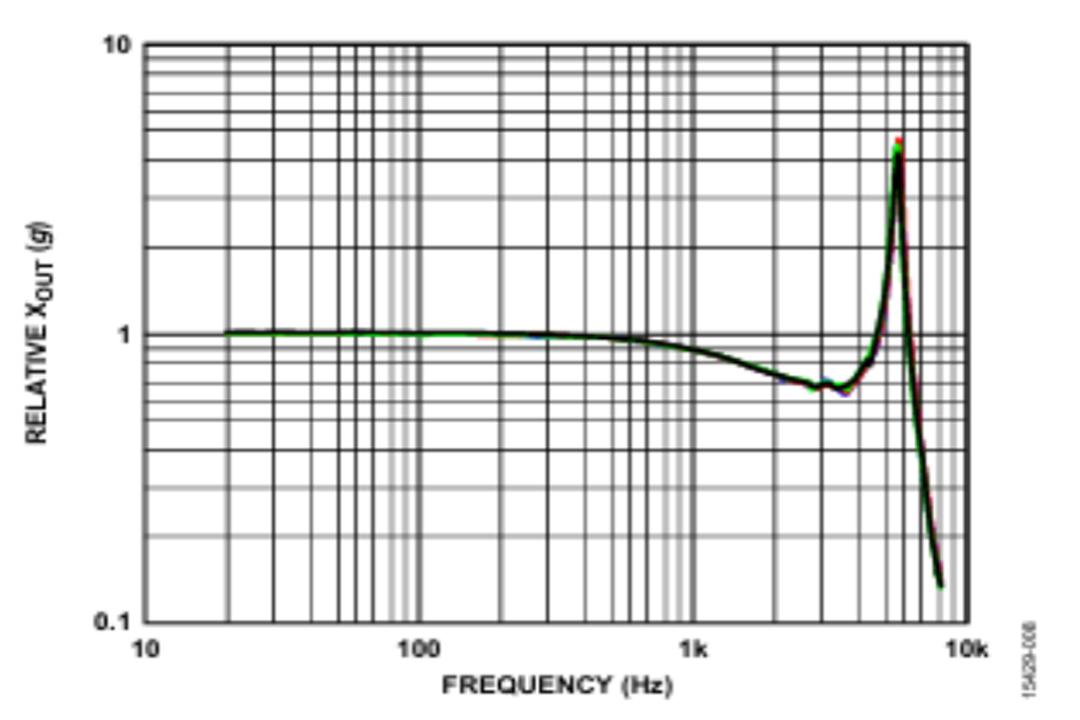
The resonant frequency of the accelerometer chip is a very important performance indicator, which is related to the operating frequency range of the sensor. 1. Definition of resonant frequency The accelerometer sensor itself is also a mechanical structure, so it also has a natural frequency. As shown in the amplitude-frequency curve in Figure 1, when the external vibration frequency is close to the resonant frequency, the sensor will resonate, and the sensitivity of the accelerometer will increase rapidly. The corresponding frequency at this time is the resonant frequency. 2. The influence of resonant frequency on sensor performance The smaller the sensor size, the higher the resonant frequency. The upper limit frequency of the accelerometer depends on the resonant frequency in the amplitude-frequency curve. Generally, the operating frequency range of the accelerometer sensor is less than 1/3 of its own resonant frequency. When the measured vibration frequency is much lower than the resonant frequency, the signal output of the accelerometer is proportional to the measured acceleration. 3. Factors affecting the resonant frequency As mentioned above, if the resonant frequency of the sensor chip is increased, the operating frequency range can be widened, the flat frequency band of the sensor will become wider, the working range will become larger, the accelerometer can be used in more scenarios, and the applicability will be better. But in fact, the increase in resonant frequency is also restricted. According to the following formula, the smaller the mass block, the larger the resonant frequency. Where f0 is the resonant frequency, K is the equivalent stiffness of the accelerometer, and M is the equivalent mass of the sensor. Therefore, the resonant frequency is a hard constraint that determines the available frequency response range of the accelerometer. Reasonable design and application require the operating frequency to be limited to less than 1/3 of the resonant frequency, and in high-precision applications, it needs to be limited to less than 1/5 to ensure linearity and reliability. The frequency response of the ADXL356 shown in Figure 2 has a resonant frequency of approximately 5.5KHz and a 3dB bandwidth of 2.5KHz. In high-precision applications, the cutoff of the low-pass filter is generally set to less than 1KHz.

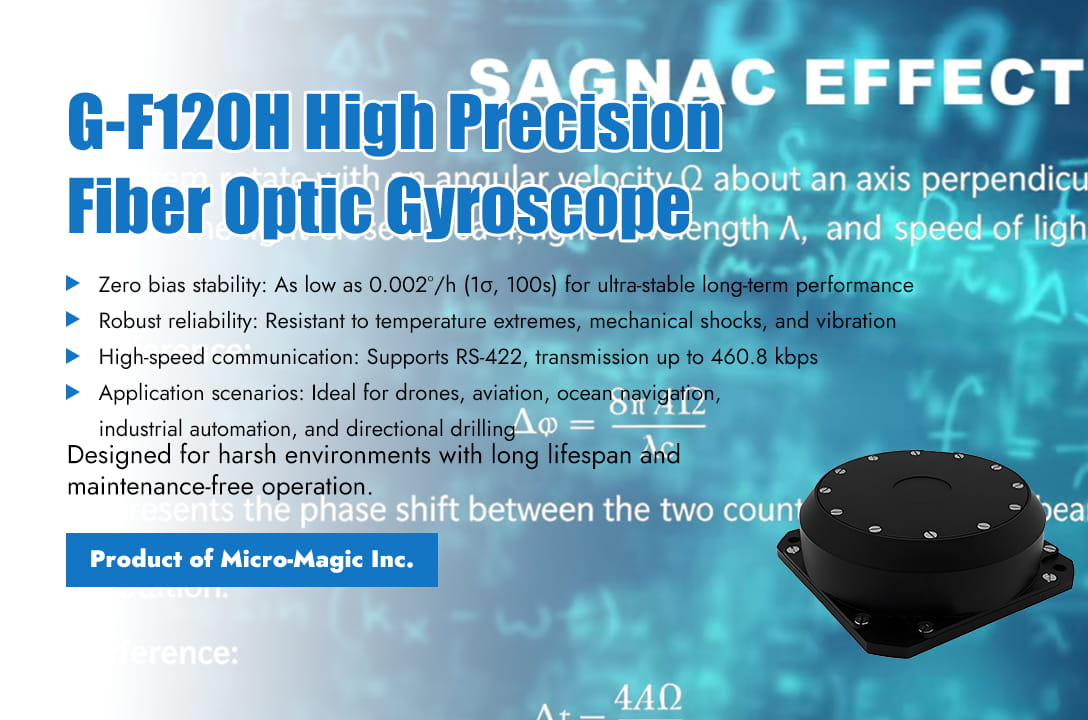
Quick preview of article content   In the field of modern navigation technology, accuracy and reliability are crucial requirements. Both military defense systems, aerospace vehicles, ocean ships and autonomous vehicle need highly accurate navigation solutions. Among numerous navigation sensors, Fiber Optic Gyroscope (FOG) has become the core component of precision navigation systems due to its unique advantages. Fiber optic gyroscope consists of a laser light source, fiber optic coil, coupler, and photodetector, and its working principle is based on the Sagnac effect. The laser is divided into two beams and propagates in the fiber coil in clockwise and counterclockwise directions, respectively. When the system is stationary, two beams of light return simultaneously and interfere destructively; When the system rotates, two beams of light will produce a phase difference, and by detecting this phase difference, the rotational angular velocity can be accurately measured.   Technical Characteristics of Fiber Optic Gyroscope   1.       High precision and high stability: Fiber optic gyroscopes do not have mechanical rotating components, avoiding the wear and drift problems of traditional mechanical gyroscopes, and have extremely high measurement accuracy and long-term stability. The drift of modern high-precision FOG can reach below 0.001/h. 2.       Quick response Due to the use of optical measurement principles, fiber optic gyroscopes have extremely fast response speeds and can detect instantaneous angle changes in real time, which is crucial for precise control of high-speed moving objects. 3.       Strong anti-interference ability Fiber optic gyroscopes have strong resistance to electromagnetic interference, vibration, and impact, making them suitable for working in harsh environments such as aerospace, military, and other applications. 4.       Long lifespan and maintenance free The design without moving parts gives the fiber optic gyroscope an extremely long service life, usually up to 10 years or more, and requires minimal maintenance, greatly reducing the cost of use. 5.       Wide dynamic range Modern fiber optic gyroscopes are capable of measuring angular velocities ranging from 0.001°/h to 1000 °/s, covering a wide range of measurement needs from extremely low to ultra-high speeds.   The Main Application Areas of Fiber Optic Gyroscope   1.              Aerospace Field Fiber optic gyroscope is a core component in navigation and guidance systems for aircraft, spacecraft, and other aircraft, used to accurately measure the attitude, angular velocity, and heading of the aircraft, ensuring flight safety and precise navigation. In the attitude control system of satellites, rockets and other spacecraft, fiber optic gyroscopes are used for attitude stabilization, orientation and control to ensure the stable attitude of the spacecraft in space. In rocket launch scenarios, it is used for tracking and measuring the rocket's launch trajectory to ensure accurate launch. 2.              Military Field   In missile guidance, fiber optic gyroscope is an important component of the missile guidance system, used to provide accurate attitude and direction information, ensuring the accuracy of missile hits. On military vehicles such as tanks and armored vehicles, fiber optic gyroscopes are used to provide attitude and direction information for navigation, control, and artillery aiming. In submarine navigation, the inertial navigation system used for submarines provides accurate position and attitude information. 3.              Other Application Areas Fiber optic gyroscope can be used for ship navigation, providing accurate heading, attitude, and angular velocity information for ship navigation and control. In fields such as oil exploration and mineral exploration, fiber optic gyroscopes are used to measure the inclination and displacement of the ground, for geological exploration and drilling guidance. For example, in directional drilling operations, fiber optic gyroscopes are used to measure the precise orientation and inclination angle of drill bits, helping to achieve complex wellbore trajectory control. In the field of industrial automation, fiber optic gyroscopes are used for attitude control and motion tracking of robots, positioning and control of precision instruments, etc. The Development of Fiber Optic Gyroscope   1.              Integration and Miniaturization   With the development of micro optics and integrated optics technology, fiber optic gyroscopes are moving towards smaller size and lower power consumption, making them applicable to more portable and embedded systems. As a leading inertial sensor design and manufacturer in China, Micro-Magic Inc has developed a series of integrated fiber optic gyroscope products (G-F50,G-F70, G-F80, G-F98, G-F120) to meet various customer needs. 2.              Multi Axis Integration The traditional single axis FOG is evolving into a two axis, three-axis integrated IMU (Inertial Measurement Unit), providing a more complete solution for measuring motion information. Micro-Magic Inc provides G-F2X70, G-F2X64 series two axis fiber optic gyroscope products and G-F3X35, G-F3G70, G-F3G90, G-F3X112 series three-axis fiber optic gyroscope products. 3.              Performance Improvement By improving fiber optic materials, optimizing optical design, and adopting digital signal processing technology, the accuracy and stability of modern fiber optic gyroscopes continue to improve. Taking the G-F120H high-precision fiber optic gyroscope produced by Micro-Magic Inc as an example, advanced integrated optical technology and FPGA closed-loop circuit design have been adopted to achieve higher accuracy, noise control, and efficiency than similar technologies. The zero bias stability is as low as 0.002 °/h (1σ, 100s), and the random walk coefficient is ≤ 0.001 °/√hr.    Conclusion   Fiber optic gyroscope, as the core sensor of modern precise navigation, plays an irreplaceable role   in key fields such as military, aerospace, marine, and autonomous driving due to its high precision, high reliability, and strong anti-interference ability. With the continuous advancement of technology, fiber optic gyroscopes are developing towards higher performance, smaller size, and lower cost, and their application scope will further expand. In future intelligent and autonomous navigation systems, fiber optic gyroscopes will continue to maintain their core position, providing precise directional guidance for human exploration and movement.

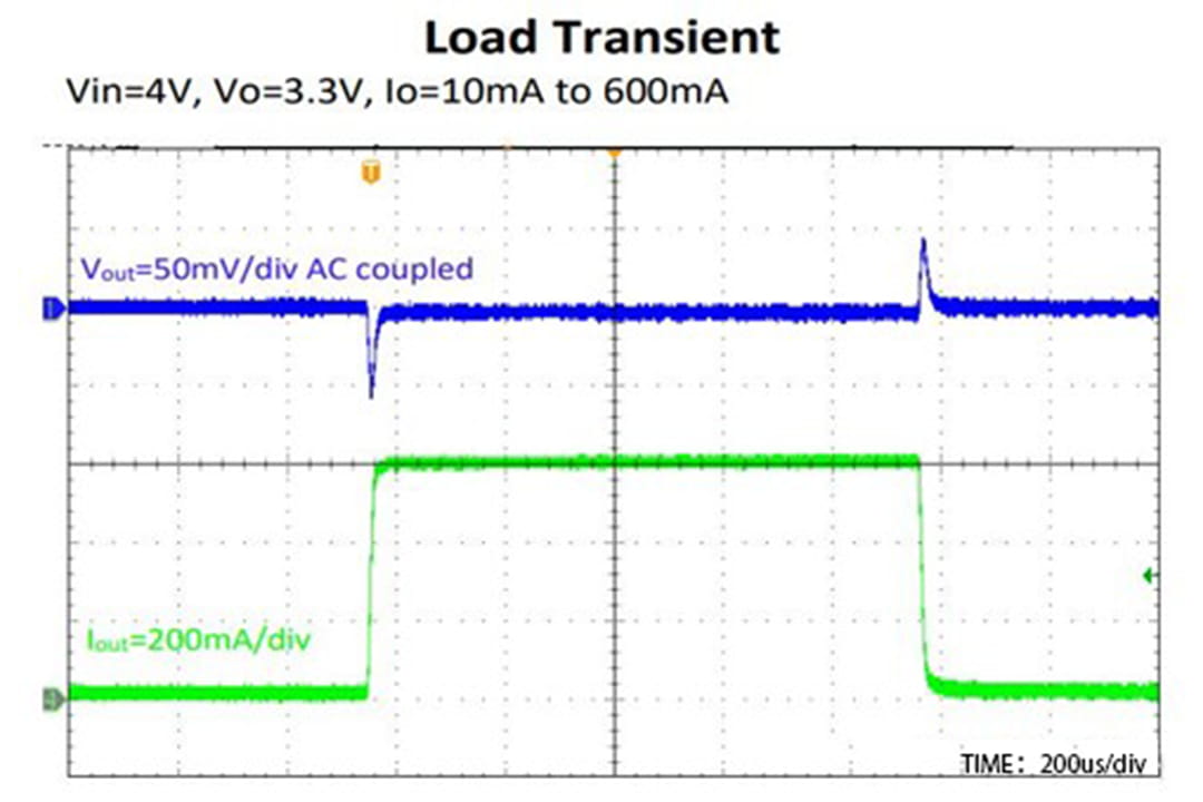
Load regulation refers to the change in output voltage when the load current is adjusted from a minimum value to a maximum value while the input voltage remains unchanged, that is, the ability to maintain a stable output voltage when the load current changes steadily. It is a steady-state indicator. The output load regulation indicator is usually expressed in mV in the LDO specification. From the definition, it can be seen that the smaller the load regulation, the better. When the load current changes suddenly, the smaller the output voltage change caused, the better the LDO performance. For LDO power supply, its output voltage is different under different load current conditions. For example, assuming that the load current of a certain LDO changes from 10mA to 300mA, the output voltage changes from 3.3V to 3.28V, that is, when the load current is 10mA, the output voltage is 3.3V; when the load current is 300mA, the output voltage is 3.28V. If the load regulation is expressed in mV, it is 3.3V-3.28V=0.02V=20mV. This means that when the load current is within 10mA~300mA, the maximum output voltage change does not exceed 20mV. Output capacitors of different sizes have different load regulation rates. The larger the output capacitor, the more stable the output voltage will be. In the figure below, when the green Iout suddenly rises, the LDO output has an undershoot, which is the load regulation rate.

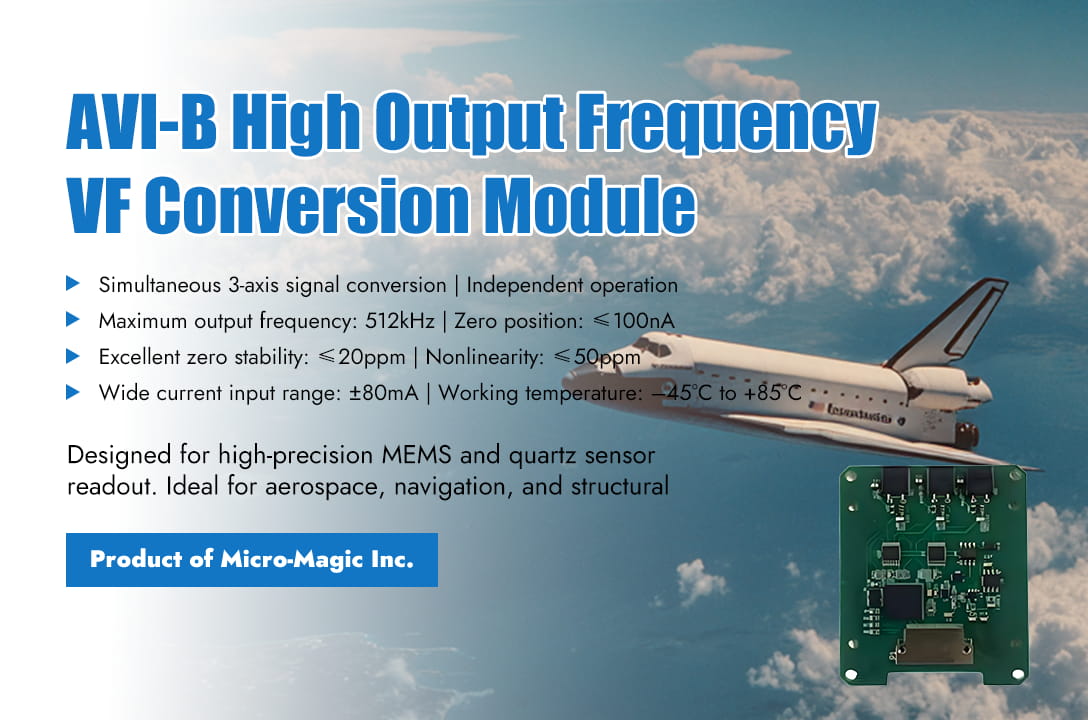
One minute to read the key points of the article Application of Current Frequency Conversion Module in Inertial Sensor System   The charge-integration I/F module plays a crucial role in inertial sensor (especially capacitive MEMS inertial sensor) measurement systems, particularly in applications demanding high precision, low noise, and wide dynamic range. Its core value lies in directly and high fidelity converting the weak charge signal output by the sensor into a digital frequency signal. The following introduces the typical applications and advantages of the charge integrator I/F module in inertial sensor systems:   Capacitive MEMS Accelerometer/Gyroscope Signal Readout   The charge integrator I/F module is used to detect small capacitance changes in the output signals of MEMS inertial sensors (accelerometers, gyroscopes). It directly measures charge and is extremely sensitive to charge changes at the fC (flying coulomb) level, capable of detecting extremely small inertial forces. The integration process itself is a low-pass filter, which can effectively suppress high-frequency noise. Using frequency signals as output, it is insensitive to amplitude noise and interference on the transmission path, making it suitable for long-distance transmission or use in noisy environments.   High Precision/Force Balanced(Servo/Force-Feedback) Inertial Sensor   In the highest precision inertial sensors, such as navigation grade MEMS or quartz beam accelerometers, a force balance closed-loop working mode is commonly adopted. The detected small displacement (sensed through capacitance/charge changes) is converted into feedback force, which is applied back to the mass block to keep it near zero. In this design process, the I/F module plays a dual role as the driver source for front-end detection and feedback DAC. Achieved ultra-high precision, stability, and precise force control. At the same time, it simplifies the closed-loop control architecture, enabling the entire closed-loop system to be efficiently implemented in the charge/frequency/digital domain.   Typical Application Scenarios   l  High precision navigation and positioning: high-precision inertial navigation systems and inertial measurement units for aviation, aerospace (satellites, rockets), ships, and land vehicles. The requirements for zero bias stability, noise, and scale factor linearity are extremely high. l  Earthquake monitoring and geophysical exploration require the measurement of extremely weak ground vibrations (as low as μg acceleration), with strict requirements for low-frequency noise and dynamic range. l  Industrial automation and robotics: precision motion control, platform stability, vibration monitoring. l  Structural health monitoring: detection of small deformations and vibrations in large buildings, bridges, and dams. l  Automotive electronics: advanced driving assistance systems, high-performance MEMS IMUs required for autonomous driving.   I/F Conversion Module Products   As an inertial sensor designer and manufacturer, Micro-Magic Inc has designed and manufactured a series of high-precision inertial sensor products, such as quartz flexible accelerometers, fiber optic gyroscopes, IMUs, INS, North Seeker, and inclinometers. At the same time, AVI series charge integration I/F (V/F) module products have also been developed in conjunction with it.   AVI-F  AVI-E  AVI-B Performance Index Specification AVI-F AVI-E AVI-B Unit Maximum output frequency 256 512 512 kHz Zero position F0 10 20 100 nA Zero stability 5 5 10 ppm Scale factor temperature coefficient 1 0.5 1 ppm/℃ Scale factor asymmetry 10 30 30 ppm Scale factor comprehensive nonlinearity 15 30 30 ppm Small signal error 0.2 0.5 0.5 Hz                         Conclusion   The charge integrator I/F module is one of the key technologies for achieving high-performance and high-precision signal readout of capacitive inertial sensors, especially MEMS accelerometers and gyroscopes. It is an essential core component in advanced inertial measurement applications that require extremely low noise, ultra-high linearity, wide dynamic range, and digital closed-loop control, providing a critical signal chain solution for high-end inertial sensors at the navigation, tactical, and even some industrial levels. With the advancement of MEMS technology and readout circuit technology, readout schemes based on charge integration principle continue to play an important role in the field of high-performance inertial sensors. AVI-B AVI-E AVI-F  

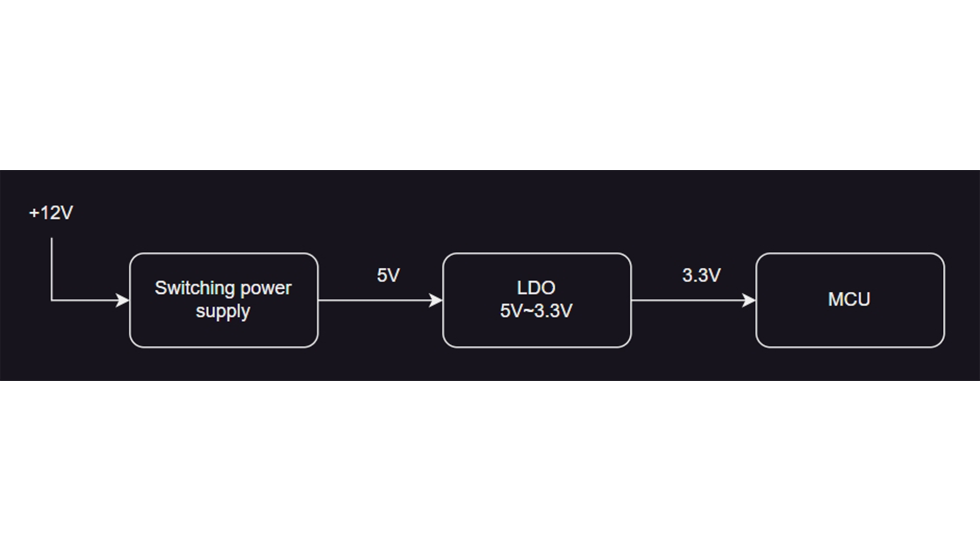
Power Supply Rejection Ratio (PSRR) refers to the ratio of the input ripple voltage to the output ripple voltage, in decibels (dB), and its expression is: The significance of PSRR lies in quantifying the degree of transmission of changes in the power input to the output. For example, if the PSRR of a certain circuit is 60dB, then for every 1V change in the power supply input voltage, the output will only fluctuate by 1mV. This indicator is particularly important in analog circuits (such as op amps, voltage regulators) because power supply noise can directly lead to signal distortion or system performance degradation. The factors affecting the PSRR of the LDO power supply are not only related to the ripple frequency, but also to the load current, input and output voltage difference, and output capacitor capacitance value. Specifically, it is reflected in: the smaller the voltage drop, the larger the load current, the higher the frequency, and the smaller the output capacitor, the lower the PSRR. Therefore, when a high common mode rejection ratio is required, it is necessary to appropriately increase the voltage difference, increase the output capacitor and reduce the load current. Figure 1 shows a schematic diagram of the relationship between the PSRR and frequency of the AP2210 ultra-low dropout difference power supply chip. From the diagram, it can be seen that its PSRR can reach 75dB at low frequency. Picture 1  PSRR vs Frequency Usually, the LDO power supply has a high PSRR, so the output ripple is low. Therefore, when designing the power supply circuit of the sensor, especially the sensor with analog output, in order to ensure the accuracy of the sensor, a low-noise and small ripple LDO is usually used to power the sensor. The output ripple of the switching power supply is large and is greatly affected by the load size. In terms of efficiency, the switching power supply is higher than that of LDO and has a smaller heat generation. Therefore, the switching power supply is generally used in combination with LDO, and the high power supply suppression ratio of LDO is used to suppress the output ripple of the switching power supply.

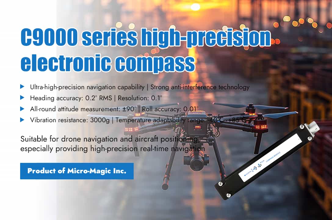
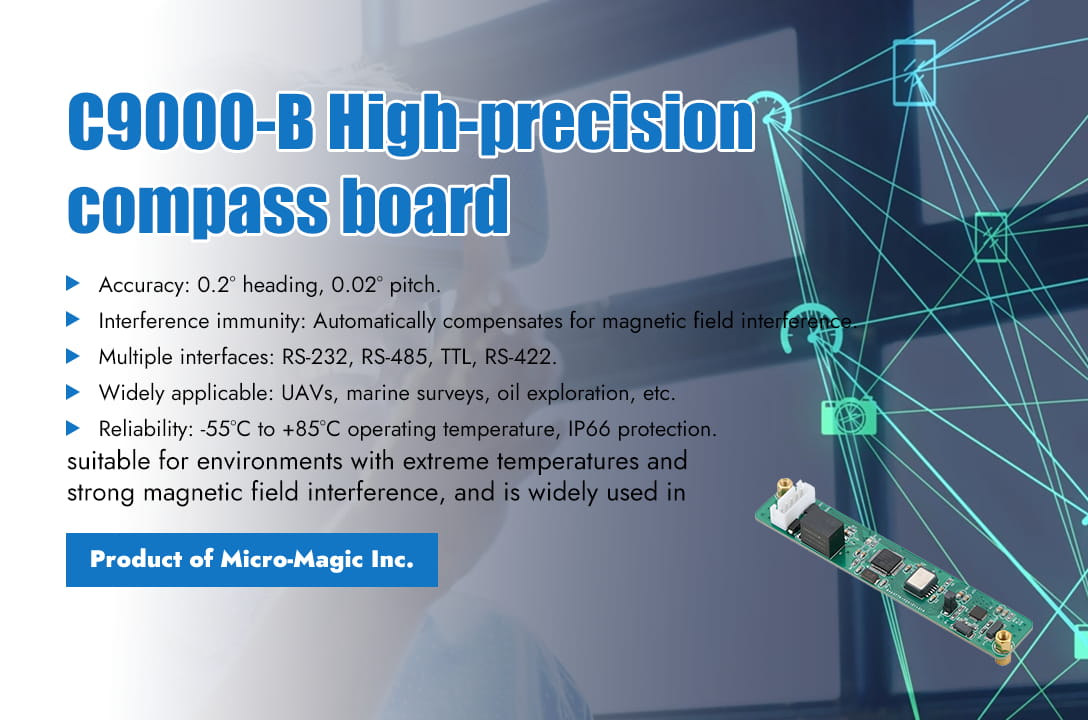
In the core field of autonomous navigation for unmanned aerial vehicles, the accuracy, reliability, and stability of direction perception directly determine the success or failure of the mission. The C9000 series high-precision six axis full attitude electronic compass launched by Micro-Magic Inc provides accurate attitude perception solutions for unmanned aerial vehicles and aircraft in all weather and terrain conditions, with military grade technical standards and industrial grade design, endowing devices with the intelligent eye of "perception direction". The C9000 series is composed of industrial grade microcontrollers with high reliability and strong anti-interference ability, high-precision tilt sensors, three-axis flux gate sensors with integrated patented technology, and driver chips. The self-developed hard and soft magnetic calibration algorithms enable the compass to eliminate the influence of magnetic fields through calibration algorithms even in environments with magnetic field interference. By integrating magnetometers for geomagnetic field measurement and accelerometers for dynamic compensation, sub-degree heading accuracy can be achieved in complex electromagnetic environments, solving the problem of attitude reference when GPS signals are obstructed. In autonomous flight of unmanned aerial vehicles, the C9000 series six axis electronic compass can correct heading drift caused by magnetic interference in real time, and use a patented tilt compensation algorithm to compensate for large range of tilt angles, ensuring flight stability and providing real-time high-precision navigation information even in extremely harsh environments.   The advantages of the C9000 series high-precision compass are mainly reflected in the following aspects:   1.       Ultra high precision navigation capability By capturing the horizontal component of the Earth's magnetic field through a magnetic sensor and combining it with a patented tilt compensation algorithm, heading compensation is applied to a large range of tilt angles, achieving a heading accuracy of 0.2° RMS (pitch angle <85°) and a resolution of 0.1°. In attitude tilt perception measurement, the pitch/roll accuracy reaches 0.01° (small tilt angle), supporting full attitude coverage of ± 90°. Eliminating heading angle drift caused by magnetic interference through bias tracking algorithm, and real-time solving complex motion attitude through extended Kalman filtering to ensure the stability of dynamic flight.   2.       Breakthrough in anti-interference technology The three-axis flux gate sensor with integrated patented technology, combined with hard/soft magnetic adaptive calibration function, automatically adapts to changes in the surrounding magnetic field environment during operation. According to pre-set algorithms, the magnetic field data collected by the sensor is analyzed and processed, and the measurement parameters are automatically adjusted to eliminate the influence of magnetic field changes, thereby ensuring that the output heading information is always accurate and reliable.   3.       Industrial grade robust design The C9000 series high-precision compass can operate in a wide temperature range, ensuring stable operation at extreme temperatures ranging from -40℃ to +85℃. The C9000 series has high resistance to vibration and impact, with a mechanical impact protection capacity of 3000g, and has passed the rigorous test of GJB150 military environmental test (high temperature/low temperature/rain/sand/vibration). Supports IP67 protection level (customizable IP68), fearless of wind, rain, sand and dust.   Product performance   Parameter   C9000-A Compass heading parameters Heading accuracy 0.3~0.5° (RMS, pitch<85°) Resolution 0.1° Repeatability 0.05° Compass inclination parameters Pitch accuracy 0.1° Roll accuracy 0.01° (pitch<15°) 0.02° (pitch<50°) 0.05° (pitch<80°) Inclination angle resolution 0.005° Inclination range Pitch ±90°; Roll 360° Calibration Hard iron calibration Yes Soft iron calibration Yes Tilt calibration Yes Physical properties Size L125*W22*H24 (mm) Weight 110g RS-232/RS485 interface connector 5-pin aviation connector Interface features Startup delay <50ms Maximum sampling rate 50 times/second RS-232 communication rate 2400~19200 baud rate RS-485 communication optional TTL communication optional Output format hexadecimal Power supply Support voltage DC+5V (9~36V) Current (max) 40mA Working mode 30mA Environment Storage range -40℃~+125℃ Working temperature -40℃~+85℃ Vibration resistance 3000g   C9000-A      

In order to prevent the power supply user from accidentally connecting the input power line incorrectly and causing the power supply to burn out, an anti-reverse connection circuit is generally required at the power supply input end. At the same time, in order to ensure that the input voltage is within a safe range, the input voltage also needs to be protected against overvoltage cutoff. The circuit shown in Figure 1 realizes the integrated function of anti-reverse connection and overvoltage protection. Its overvoltage protection function is analyzed as follows: When Vin is in the normal input voltage range, the voltage regulator Z1 does not reversely break down, the current of R2 and R3 is basically 0, the Vbe of the transistor P1 is 0, that is, the PNP transistor is not turned on, and the Vgs of the PMOS tube Q1 is determined by the voltage divider of resistors R4 and R5. Vgs is greater than the conduction threshold, and the PMOS tube is turned on, that is, the power supply works normally; when the Vin input is greater than the normal input voltage, at this time Vin>Vbr, the voltage regulator is broken down, the PNP transistor Q1 is turned on, VCE≈0, that is, the Vgs of the PMOS tube is ≈0, and the PMOS tube is turned off, that is, overvoltage protection is achieved. Its reverse connection protection function is analyzed as follows: the input reverse connection protection is realized by NMOS tube Q2. When the positive pole of the power supply is input from Vin, the gate voltage Vgs of NMOS tube Q2 is high. At this time, Q2 is turned on, Q1, load RL and Q2 form a loop, and the circuit works normally; when the positive pole of the power supply is reversed from the negative terminal below, Q2 is cut off, the entire loop is disconnected and the circuit does not work, thereby playing a role in reverse connection protection.

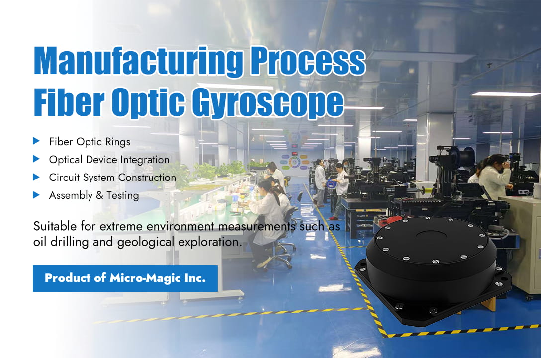
Fiber optic gyroscope has become the preferred core component for high-precision and high reliability inertial navigation systems due to its significant advantages such as all solid state design, no moving parts, fast start-up, long lifespan, wide dynamic range, and strong resistance to impact and vibration. However, behind the outstanding performance of fiber optic gyroscopes is their extremely precise and complex manufacturing process. From the selection and processing of specialized optical fibers, the coupling and alignment of precision optical components, to the precision winding and curing of the core sensing coil, and further to the integration of complex electronic systems and the implementation of sophisticated environmental compensation algorithms – each production stage embodies the crystallization of cutting-edge materials science, precision optical engineering, microelectronics technology, and advanced control theory. Even the slightest deviation during the manufacturing process can have a decisive impact on the accuracy, stability, and reliability of the final product. Below is a detailed introduction to the production process of fiber optic gyroscope. 1.       Manufacturing of fiber optic rings The core component of a fiber optic gyroscope is the fiber ring, and its manufacturing process is crucial. Firstly, high-quality optical fibers need to be selected and wound into a ring shape through precise winding processes. During this process, it is necessary to strictly control the tension of the optical fibers, the diameter and density of the winding ring to ensure the performance and stability of the fiber ring. After winding, adhesive coating and curing are performed for shape fixation. Subsequently, the fiber optic ring needs to undergo temperature cycling aging to eliminate internal residual stress and enhance mechanical stability through epoxy coating. 2.       Optical Device Integration After the fiber optic ring is manufactured, it needs to be precisely assembled with other optical components. Mainly includes the assembly of Y-waveguide modulators and the integration of light sources and detectors to ensure smooth and stable optical paths. In addition, strict performance testing of the assembled components is required to ensure that they meet the design requirements. 3.       Circuit system construction The construction of circuit systems includes the design of signal processing circuits and closed-loop feedback circuits. FPGA serves as the core processor to generate square wave/sawtooth wave modulation signals to drive the Y waveguide, bias the operating point to the sensitive area, and calculate the phase difference (Δφ) of the interference signal output by the detector, which is converted into angular velocity (Ω). Dynamically compensate for Sagnac phase difference through digital closed-loop control to improve linearity and dynamic range. 4.       Whole machine assembly and testing After completing the manufacturing of fiber optic rings, optical components, and circuit boards, the next step is to proceed with overall assembly. This process includes environmental adaptability encapsulation and performance calibration and compensation. The optical and electronic units are sealed inside a metal shielding shell to isolate temperature and humidity changes and electromagnetic interference. Military grade products use titanium alloy shells to enhance impact resistance. Subsequently, a series of tests and calibrations were conducted on the fiber optic gyroscope, including zero bias calibration, temperature compensation, and threshold testing, to ensure that all performance indicators meet the expected requirements. The key process difficulties in the manufacturing process of fiber optic gyroscopes mainly include the following: 1. Precision winding of fiber optic coils The stress generated during the winding process of fiber optic coils can cause polarization errors. The solution is to use polarization maintaining fibers and adopt a symmetrical winding process. 2. Packaging and Interconnection of Integrated Optical Chips (Y-Waveguides) Y-Waveguides are the core multifunctional integrated optical devices of FOGs. During the packaging and interconnection process, the alignment accuracy of the optical axis is extremely high. the solution to this difficulty is to use an active alignment system and a polarization maintaining fusion splicer. 3. Temperature drift Temperature changes can cause gyroscope phase drift, affecting measurement accuracy. The solution is to use multi-stage depolarizers and adopt segmented temperature compensation algorithms to eliminate the impact of temperature drift.

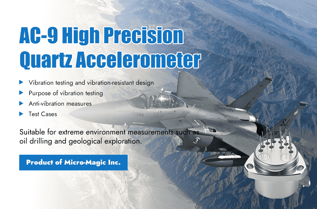
Quartz flexible accelerometers are widely used in aerospace, inertial navigation, precision measurement and other fields due to their advantages of high precision and stability. However, its core sensitive component - quartz flexible pendulum - is very fragile and extremely sensitive to vibration environments. Vibration may cause performance degradation, zero shift, and even structural damage. Therefore, strict vibration testing and effective anti vibration measures are crucial.   Purpose of Vibration Testing   The purpose of vibration testing is to evaluate the performance, structural integrity, and reliability of accelerometers in actual or expected vibration environments. The main types of testing include sine vibration testing and random vibration testing. Sine vibration testing is to find the resonant frequency of the structure and evaluate its response and tolerance at specific frequencies. Typically, within the specified frequency range (e.g., 5 Hz – 2000 Hz or higher, according to the specification), a linear or logarithmic sweep is performed along three mutually perpendicular axes. Frequencies exhibiting an abnormal increase in accelerometer output (response amplification) are recorded. Special attention should be paid to the first-order and second-order flexural resonant frequencies of the quartz flexure, as these frequencies are most prone to damage. The relationship between the input vibration and output signal is analyzed. Perform fixed frequency vibration for a specified duration (such as several minutes) on the identified resonant frequency points (especially the pendulum resonance points) to test their fatigue life and stability. Random vibration testing is to simulate wideband, random vibration excitations in actual environments (such as rocket launches, engine noise, aerodynamic turbulence, vehicle driving), and evaluate their comprehensive performance under statistically distributed vibrations. Apply vibrations with specific power spectral density patterns along three mutually perpendicular axes within the specified frequency range. The scale of testing is usually higher than that of sine testing, which can better reflect the real environment. PSD spectra and Grms values are developed based on specifications or measured data. The key monitoring parameters in the test include output signals, physical status, and performance verification. The output signal mainly observes zero offset, scale factor changes, increased noise levels, abnormal outputs (saturation, oscillation), etc; The physical state mainly involves checking whether the accelerometer has any abnormal noise, whether the structure is loose, and whether there is any damage to the appearance (after testing, the cover needs to be opened to check the swing plate); Performance validation mainly involves comprehensive static performance testing of accelerometers before, during, and after vibration (zero bias, scale factor, second-order nonlinearity, threshold, resolution, repeatability, etc.), comparing the effects of vibration.   Vibration Mitigation Measures   To address the vulnerability of quartz flexure accelerometers, vibration resistance measures must be implemented at multiple levels.   (1)      Core sensitive structure design and process Firstly, it is necessary to optimize the design of the oscillating plate. While meeting the requirements of sensitivity and bandwidth, the thickness of the oscillating plate should be appropriately increased (balancing sensitivity), the shape and support structure should be optimized, and the lowest order resonant frequency should be maximized to be higher than the expected main vibration environment frequency (ideally higher than twice). Avoid resonance frequencies falling in the main vibration energy concentration zone. Secondly, it is precision manufacturing and assembly, strictly controlling the machining accuracy and symmetry of key components such as swing plates, torque converter coils, differential capacitor plates, etc., to ensure uniform stress distribution and reduce internal stress concentration points. Reliable processes such as laser welding are used to connect the swing plates to the base. Finally, the selection of materials should be based on high-strength and high stability quartz materials, and the stiffness and damping characteristics of the base and shell materials should also be considered.   (2)      Internal mechanical isolation and damping Firstly, apply a small amount of special damping adhesive (such as silicone rubber base) on the non sensitive area of the swing plate or the supporting beam. This is one of the most commonly used and effective measures, which can significantly reduce the resonance Q value and decrease the resonance amplification factor. However, extreme caution should be taken to avoid affecting sensor performance (such as introducing thermal stress, affecting symmetry, and increasing mass). Secondly, a micro isolation system (such as low stiffness, high damping rubber pads, metal rubber, micro wire rope isolators, etc.) should be designed between the core of accelerometer (including the core components of the swing plate assembly) and the housing base to isolate the transmission of high-frequency vibrations to the sensitive core. The stiffness, damping, and load-bearing capacity need to be carefully designed.   (3)      Sealing and Filling Encapsulating silicon gel or silicone rubber with low modulus and high damping in the inner cavity of the accelerometer (usually between the core and the shell) is another very effective anti vibration measure (especially anti shock and high-frequency vibration). Silicon gel or silicone rubber provides damping and absorbs vibration energy; Support internal structure and suppress relative motion; Protect internal components from contamination and moisture. The sealing adhesive needs to have extremely low shrinkage stress, excellent thermal stability, good adhesion, low air release, and low permeability (especially for space applications). The sealing process (excluding bubbles and curing) is crucial, as poor sealing can actually introduce stress or contamination.   (4)      External installation and system level vibration isolation Optimize the installation interface to ensure that the installation base is flat and rigid. Tighten the connecting bolts evenly to the specified torque to avoid introducing local stress or reducing overall stiffness due to improper installation. At the same time, install appropriate external shock absorbers between the accelerometer and vibration sources such as engine mounts and aircraft structures. Select the type of isolator (such as metal rubber isolator, wire rope isolator, viscoelastic damping isolator) based on the characteristics of the main vibration frequency, and its natural frequency should be much lower (usually <1/√ 2 times) than the lowest main vibration frequency that needs to be isolated. The load-bearing capacity of the isolator, environmental adaptability (temperature, vacuum), and the impact on the low-frequency performance of the sensor also need to be considered.   Test cases   Taking the AC-9 series high-precision quartz accelerometer produced by Micro-Magic Inc as an example, the influence of vibration environment on the K0 index of the accelerometer is tested. Before vibration, the quartz accelerometer is in a 0g state, the product is powered on, data is collected for 1 minute, and take the average of the data, denoted as ; Start the vibration table under the following vibration conditions: 6g, random vibration at 200~2000Hz, wait for the vibration table to stabilize, collect data for 1 minute, and take the average of the data, denoted as ; Rotating vibration fixture, quartz accelerometer in 0g state, then power on the product, collect data for 1 minute, and take the average of the data, denoted as . By calculation, it can be concluded that:   Conclusion   The vibration problem of quartz flexible accelerometers is a system engineering issue that needs to be addressed throughout the entire process of design, manufacturing, testing, and application. When selecting and designing anti vibration measures, careful trade-offs must be made to ensure that the core performance indicators of the accelerometer are not significantly sacrificed while improving the anti vibration capability, and other environmental adaptability requirements are met.   AC-9