Applications

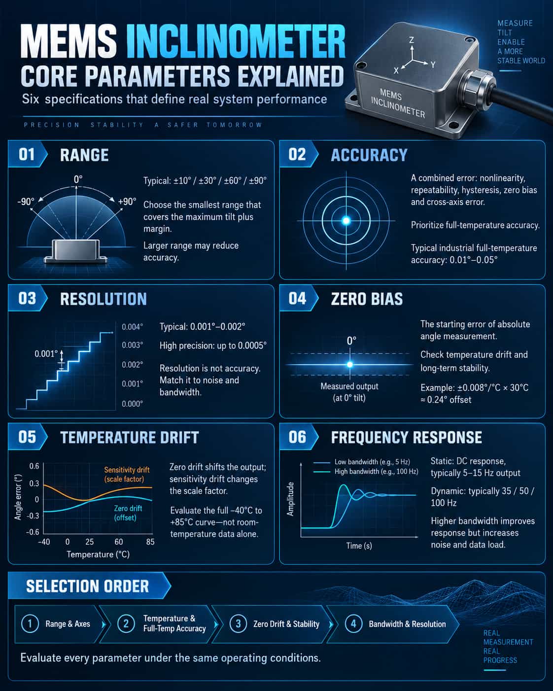
When selecting a MEMS inclination sensor, the data sheet often lists more than a dozen parameters, but the six parameters that really determine the system performance are usually the range, accuracy, resolution, bias, temperature drift and frequency response. Understanding their definitions, test conditions, and coupling relationships between them is more important than simply comparing numbers. Measuring range: bigger is not better The measuring range is the tilt angle range that the sensor can measure. Common options include ±10°, ±30°, ±60°, ±90°, etc. Some products support single-axis or dual-axis measurement. The first principle of range selection is to cover the actual maximum inclination angle and leave a safety margin, but there is usually a trade-off between range and accuracy: in the same series of products, the accuracy of the full temperature range of the ±10° range is often better than the ±90° range. This is because the nonlinearity, packaging stress and cross-axis errors of MEMS sensitive structures at large ranges are more difficult to control. Therefore, if the actual working condition only requires ±15°, it is usually more reasonable to choose the ±30° range than ±90°. In addition, the X- and Y-axis measuring ranges of dual-axis sensors may be the same, but the installation direction will affect the effective measuring axis. When selecting, make sure that the measuring axis is consistent with the mechanical axis. Accuracy: A comprehensive error concept Accuracy is often misunderstood as "error of a single measurement". In fact, it is usually absolute accuracy, including the comprehensive result of multiple errors such as nonlinearity, repeatability, hysteresis, zero deviation, and horizontal axis error. The accuracy in the data sheet must pay attention to the test conditions: there is a big difference between normal temperature accuracy and full temperature range accuracy. For example, the full temperature range accuracy of an industrial-grade digital output dual-axis inclination sensor in the range of -40°C to +85°C is 0.01° to 0.05°, but it may be better at room temperature. When selecting a model, you should give priority to the accuracy in the full temperature range, because temperature changes in outdoor and industrial sites will directly amplify the error. If the system only needs relative angle changes, part of the zero offset can be eliminated through "relative zero point" calibration, but temperature drift and nonlinearity cannot be eliminated. Resolution: being able to distinguish does not mean accurate measurement Resolution is the smallest angular change that the sensor can detect and distinguish. It is commonly 0.001°~0.002°, and high-precision products can reach 0.0005°. The resolution is mainly determined by the number of AD bits, noise level and filtering algorithm, but it is not equal to accuracy. A sensor with a resolution of 0.001° may have an actual accuracy of 0.05°. High resolution is valuable in static leveling and slow tilt monitoring, but in a vibration environment, excessive resolution will amplify noise. Therefore, the resolution should match the noise density, bandwidth and actual control needs, rather than blindly pursuing the minimum value. Zero offset: starting point error of absolute angle Zero bias is the deviation between the actual output of the sensor at the zero inclination position and the theoretical zero point. Zero offset directly affects absolute angle measurement, but can be corrected through on-site calibration or relative zero setting. What's more troublesome is the zero bias temperature drift, which is the drift of the zero point with temperature changes. The unit is usually °/℃. For example, zero temperature drift of ±0.008°/°C will introduce a zero point offset of approximately 0.24° at a temperature difference of 30°C, which cannot be ignored for high-precision tracking or safety control. The long-term stability of the zero bias is also critical, as it determines the zero drift of the sensor after one year of operation. When selecting, you should pay attention to "zero bias temperature drift" and "long-term stability", rather than just looking at the initial zero bias. Temperature drift: the key to accuracy across the entire temperature range Temperature drift is divided into zero point temperature drift and sensitivity temperature drift. The zero-point temperature drift is represented by the overall deviation of the angle output with temperature; the sensitivity temperature drift is represented by the change of the proportional factor with temperature, and the commonly used unit is ppm/℃. Modern industrial-grade MEMS inclination sensors usually have built-in temperature sensors and perform real-time compensation through polynomial fitting or look-up table methods to ensure repeatability in low and high temperature environments. But the compensation effect depends on the factory calibration quality. When evaluating temperature drift, manufacturers should be required to provide a full temperature range accuracy curve of -40°C to +85°C, rather than just looking at normal temperature indicators. If the application environment temperature changes drastically, the temperature drift index should take priority over the normal temperature resolution. Frequency response: the watershed between static and dynamic Frequency response determines whether the sensor can keep up with changes in angle. Static inclination measurement only requires DC response and an output rate of 5Hz~15Hz; dynamic measurements such as platform leveling, vibration monitoring, and tracking bracket anti-wind vibration require higher bandwidth and output rate, commonly 35Hz, 50Hz or even 100Hz. However, high output rates will bring increased noise and communication pressure. High-frequency automatic output in RS485 half-duplex mode may also affect command reception. In this case, it is recommended to use question and answer mode or increase the baud rate. Response time, start-up time and filter cutoff frequency also need to be considered: too much filtering will cause lag, and too light filtering will cause loud noise. In engineering, moving average or low-pass filtering is usually performed on the controller side to strike a balance between response speed and noise suppression. Parameter coupling and selection sequence The six parameters are not independent: the measurement range affects the accuracy, the temperature drift affects the accuracy in the full temperature range, the resolution is restricted by noise and bandwidth, and the zero-bias temperature drift determines long-term stability. A reasonable selection sequence is: first determine the range and number of measurement axes, then clarify the operating temperature range and full temperature zone accuracy requirements, then look at the zero bias temperature drift and long-term stability, and finally select the output rate and resolution based on the control bandwidth. Interfaces, protection levels, and shock and vibration resistance are additional conditions at the system integration level. To sum up, the key to analyzing the core parameters of MEMS inclination sensors is not to remember the numbers, but to understand the definition, test conditions and engineering impact of each parameter. The measuring range must match the actual tilt angle, the accuracy depends on the full temperature range, the resolution must be balanced with noise and bandwidth, the zero bias and temperature drift determine long-term reliability, and the frequency response determines dynamic applicability. Only by comprehensively evaluating these parameters in the same application scenario can the inclination sensor that is truly suitable for the system be selected.

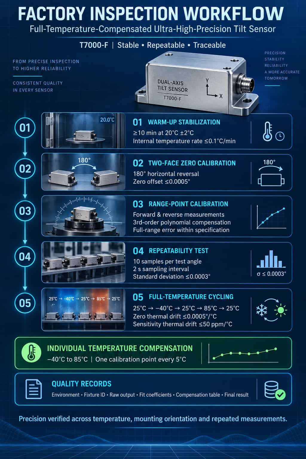
Indicated value error and repeatability are the core performance indicators for ultra-high-precision inclinometers featuring full-temperature compensation: the former reflects the deviation between the reading at a specific angle and the true angle, while the latter reflects the consistency of measurements taken multiple times under identical conditions. Using the T7000-F as an example, this article outlines its factory inspection process—covering warm-up stabilization, zero-point calibration via the dual-side method, full-scale point calibration, repeatability testing, and full-temperature cycling—to ensure stable, repeatable, and traceable output across varying temperatures, mounting surfaces, and measurement conditions. 1. Core Indicators and Inspection Logic The T7000-F utilizes MEMS sensing technology and full-temperature compensation algorithms to achieve an absolute accuracy of 0.001° within a ±5° measurement range. For products of this class, factory inspection must go beyond single-point output checks at room temperature; instead, a comprehensive testing sequence centered on "indicated value error" and "repeatability" is required. The inspection process typically includes static warm-up, zero-point calibration, full-scale point calibration, repeatability verification, and full-temperature cycling. Raw data, environmental conditions, and pass/fail results are recorded at each stage to create traceable quality records. 2. Warm-up Stabilization After power-on, the sensor must remain undisturbed for at least 10 minutes, during which no commands are sent. The ambient temperature is maintained at 20°C ± 2°C. Real-time monitoring of the internal temperature sensor confirms that the rate of temperature change does not exceed 0.1°C/min. Additionally, the difference in zero-point output between the start and end of the warm-up period is recorded as a characteristic parameter of the device's "thermal stabilization time." The purpose of warm-up stabilization is to eliminate the impact of initial thermal transients on the MEMS sensing element and internal circuitry. For ultra-high-precision inclinometers, insufficient warm-up directly introduces zero-point drift, leading to distorted data in subsequent calibration and testing. 3. Zero-Point Calibration via Dual-Side Method The T7000-F is mounted on a Grade 0 surface plate with a flatness tolerance of no more than 0.005 mm. With the sensor facing upward, the X- and Y-axis outputs are recorded; the sensor is then rotated 180° horizontally around its vertical axis, and the X- and Y-axis outputs are recorded again. The zero-point error for each axis is calculated based on these two sets of readings. The acceptance criterion is that the zero-point deviation, calculated using the dual-sided method, must not exceed 0.0005°. If the zero-point deviation exceeds the limit, the sensor structure is typically deemed abnormal—potential causes include misalignment of the internal sensitive axis or abnormal packaging stress—requiring the unit to be returned for re-inspection. The dual-sided method effectively isolates the sensor's intrinsic zero-point error from errors caused by mounting surface tilt or fixture references, making it a critical step in the zero-point calibration of ultra-high-precision inclinometers. 4. Full-Scale Point Calibration Full-scale point calibration is performed using a high-resolution optical indexing head. The T7000-F is rigidly mounted onto the indexing head's platform, ensuring the sensor's sensitive axis is perpendicular to the indexing head's axis of rotation. The indexing head is rotated to target angles in both forward and reverse directions; the T7000-F's output value is recorded after a 5-second stabilization period. Polynomial fitting—typically using a third-order polynomial—is applied to the indicated value errors from both forward and reverse rotations. The resulting fitting coefficients are written to the sensor to implement non-linearity compensation. Ultimately, the indicated value error across the entire measurement range must not exceed the accuracy specification. Measuring in both directions is essential to capture hysteresis error—the difference in output for the same input angle between the forward and reverse strokes. This stage embodies the core logic of the factory inspection for ultra-high-precision inclinometers with full-range temperature compensation: it goes beyond merely verifying compliance to ensure—through fitting and compensation—that each unit achieves its nominal accuracy during actual operation. 5. Repeatability Test The repeatability test verifies the consistency of sensor measurements taken multiple times under identical conditions and angles. The indexing head is set to three typical angles: zero position (0°), mid-range (+15°), and full-scale (+30°). Ten consecutive samples are taken at each angle with a 2-second interval between samples; output values are recorded, and repeatability is calculated based on the root-mean-square error (RMSE). The acceptance criterion is that the standard deviation of repeatability ($s$) must not exceed 0.0003°. If this limit is exceeded, potential causes include loose mechanical connections, excessive power supply noise, or anomalies in the MEMS sensing element. Repeatability testing serves as a crucial basis for evaluating sensor short-term stability and fixture reliability; it is also a key step in factory inspection for distinguishing between "accurate in a single instance" and "consistently reliable" performance. 6. Full-Temperature Cycling Test For MEMS inclinometers, the primary source of error is typically temperature rather than nonlinearity. Consequently, full-temperature cycling tests are conducted to verify the sensor's temperature characteristics. During the test, the T7000-F is fixed at a non-zero angle (e.g., +10°) without altering the mechanical angle throughout the process. Angle outputs are recorded at specific temperature points—25°C, -40°C, 25°C, 85°C, and a return check at 25°C—to calculate zero-point temperature drift and sensitivity temperature drift. Acceptance criteria are set as follows: zero-point temperature drift ≤ 0.0005°/°C; sensitivity temperature drift ≤ 50 ppm/°C. These specifications are not derived from theoretical calculations but are based on actual measurements and compensation data obtained for each individual chip. A temperature compensation table is generated for every sensor, covering the range from -40°C to 85°C with compensation points set every 5°C; real-time interpolation is used for compensation during operation. Full-temperature cycling is a core step in the factory inspection of products featuring full-temperature compensation. Only through actual measurements across the entire temperature range, the creation of individualized compensation tables, and real-time firmware application can the sensor maintain ultra-high precision output across a wide temperature range. 7. Evaluation, Compensation, and Traceability Upon completion of the aforementioned tests, a comprehensive evaluation is performed for each sensor. Inspection records must include the ambient temperature, fixture ID, dividing head reading, raw output, curve-fitting coefficients, the temperature compensation table, and the final pass/fail result. Non-conforming units are categorized by the type of anomaly—such as structural, assembly, electrical noise, or sensing element issues—and subjected to appropriate rework or re-inspection procedures. In summary, the factory inspection process for the T7000-F demonstrates that quality control for ultra-high-precision inclinometers with full-temperature compensation is not merely a test of isolated metrics, but a complete closed-loop process covering thermal stability, zero-point accuracy, measurement range, repeatability, and temperature characteristics. The ultimate objective is to ensure that angle outputs remain stable, repeatable, and traceable across varying temperatures, mounting surfaces, and repeated measurement cycles. This process offers a general reference for similar ultra-high-precision inclinometers featuring full-temperature compensation.

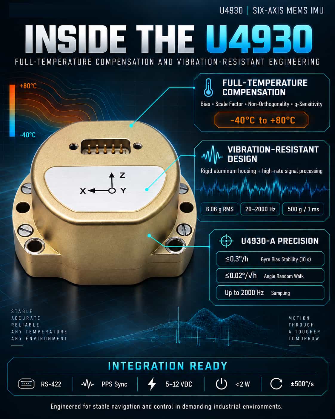
As industrial drones, autonomous driving systems, and high-precision navigation systems increasingly demand compact size, high performance, and low cost, MEMS Inertial Measurement Units (IMUs) are steadily advancing toward tactical-grade—and even navigation-grade—performance. The U4930 series of six-axis MEMS IMUs from Micro-Magic delivers a highly competitive solution, featuring robust full-temperature compensation technology, superior vibration resistance, and compatibility with leading international products (such as the HG4930).   Core Technology: Full-Temperature Compensation and System Calibration   One of the most critical sources of error in MEMS inertial devices is the drift in bias and scale factor caused by temperature fluctuations. Without effective compensation, even minor temperature changes can lead to massive errors in navigation calculations—a classic case of "a miss is as good as a mile." The U4930’s standout feature is its sophisticated compensation algorithm covering the entire operating temperature range (-40°C to +80°C). The system performs comprehensive temperature-based compensation for the bias, scale factor, non-orthogonality errors, and acceleration-dependent terms of both the gyroscope and accelerometer. This goes beyond simple linear correction; it relies on a complex error model established through extensive testing in environmental chambers. Consequently, the U4930-A model achieves a full-temperature bias stability of ≤0.3°/h (10s smoothing) and an angular random walk of ≤0.02°/√h. These specifications enable the system to maintain exceptional attitude accuracy during short periods without external aids (such as GNSS)—a capability that is crucial for navigation in tunnels, underground environments, or underwater.   Mechanical Robustness: Vibration and Shock Resistance   Harsh mechanical environments—characterized by high dynamics or vehicle/airborne mounting—pose another major challenge for MEMS IMUs. Intense vibration can introduce spurious angular velocity through mechanical coupling, causing attitude calculation errors to diverge. The U4930 addresses this with a robust structural design. Encased in a lightweight, high-strength aluminum alloy housing, the unit withstands random vibration of 6.06g (RMS) across the 20–2000 Hz range and shocks of 500g/1ms. Coupled with high-speed sampling (up to 2000 Hz) and synchronous processing capabilities, the U4930 leverages high-bandwidth data to effectively filter out vibration noise in the time domain, ensuring the output of stable, accurate motion data even amidst the intense shaking of rotor-wing drones or the jolting of vehicles.   Strategic Positioning: A Seamless Drop-in Replacement for the HG4930   The U4930’s most ingenious feature is its strategic market positioning: it is fully compatible with Honeywell’s classic HG4930 IMU. This compatibility extends beyond physical dimensions and M4 screw mounting to include the RS422 differential interface and PPS synchronization signal definitions. Users can upgrade directly without modifying existing carrier boards or power architectures (supporting 5–12V input and <2W power consumption), gaining a wider gyroscope measurement range (±500°/s vs. ±400°/s) and superior noise performance.   In summary, the U4930 is far more than a mere assembly of components. It eliminates temperature drift through system-level full-temperature compensation, resists vibration interference via a high-rigidity structure and high-speed sampling, and lowers the barrier to adoption through seamless hardware compatibility. For navigation and control systems demanding high reliability, this robust technical design and implementation embody the product's core value.

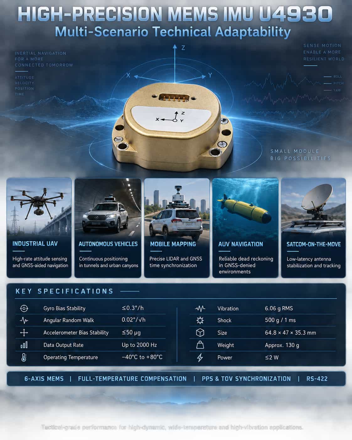
High-precision Inertial Measurement Units (IMUs) are core sensors for attitude sensing and autonomous navigation in moving platforms. In complex application scenarios—such as industrial drones, autonomous driving, mobile mapping, and underwater navigation—systems impose rigorous requirements regarding IMU accuracy, dynamic response, environmental resilience, and data synchronization capabilities. The U4930 series six-axis MEMS inertial measurement module from Micro-Magic Inc. offers a mature and reliable inertial sensing solution for these applications, featuring tactical-grade inertial specifications, precise full-temperature compensation, high-bandwidth output, and a compact, lightweight design.   **Key Technical Features of the U4930**   The U4930 integrates a high-performance three-axis MEMS gyroscope and a three-axis MEMS accelerometer. It features internal calibration and compensation across the full operating temperature range (-40°C to +80°C) for bias, scale factor, non-orthogonality errors, and acceleration-sensitive terms. The gyroscope offers a measurement range of ±400°/s to ±500°/s (depending on the model), with bias stability (10s smoothing) better than 0.3°/h and angular random walk as low as 0.02°/√h. The accelerometer features a ±30g range, bias stability better than 50μg, and velocity random walk ≤0.03 m/s/√h. The module measures just 64.8 × 47 × 35.3 mm and weighs approximately 130g, with a steady-state power consumption of ≤2W. It supports data output rates up to 2000Hz and offers robust performance, including 6.06g RMS vibration resistance and 500g/1ms shock resistance.   These specifications demonstrate that the U4930 achieves tactical-grade MEMS IMU standards, capable of maintaining measurement accuracy under harsh conditions—such as high dynamics, wide temperature ranges, and intense vibration—thereby laying the foundation for its deployment across diverse application scenarios. Technical Adaptation Analysis for Typical Application Scenarios   (1) Industrial Drones: High-Dynamic Attitude Reference and Dead Reckoning   Industrial drones require real-time, high-update-rate attitude data (roll, pitch, and yaw) for stable flight control and autonomous navigation. The U4930’s 2000 Hz data output rate ensures precise capture of the airframe's transient angular motion, while its angular random walk (as low as 0.02°/√h) effectively suppresses the rate of attitude integration drift. The module supports time synchronization with GNSS receivers (via PPS input and GPRMC message parsing), enabling loosely or tightly coupled integrated navigation; it maintains trajectory continuity through pure inertial dead reckoning during brief GNSS signal outages—a capability critical for tasks such as power line inspection and long-endurance surveying.   (2) Autonomous Vehicles: Continuous Positioning in Complex Operating Conditions   For autonomous vehicles operating in environments where GNSS signals are obstructed—such as urban canyons, tunnels, and underground parking garages—the IMU becomes the core component for dead reckoning. The U4930’s bias stability (0.3°/h) and low-noise characteristics ensure that positional drift remains within acceptable limits over periods of tens of seconds. Its full-temperature-range compensation mechanism guarantees consistent performance despite temperature fluctuations in the engine compartment (-40°C to 80°C), while its 6.06g vibration resistance effectively mitigates measurement disturbances caused by road bumps and engine vibrations. A tiered precision lineup (Models A, B, and C) allows systems ranging from L2+ to L4 autonomy—and with varying budget constraints—to access inertial performance tailored to their specific needs.   (3) Mobile Mapping and Track Inspection: High-Precision Spatiotemporal Reference Synchronization   Vehicle-mounted or airborne LiDAR systems require IMUs to provide high-precision attitude and position references to ensure the accuracy of 3D point cloud registration. The U4930’s low angular random walk (≤0.02°/√h) directly translates to reduced point cloud drift, a factor that is particularly crucial for long-distance data acquisition missions. Additionally, its TOV differential synchronous pulse output and PPS input capabilities enable strict synchronization between IMU sampling moments and GNSS one-pulse-per-second (PPS) signals, providing precise trigger signals for point cloud timestamping. In railway track inspection, the module can be integrated with an odometer and GNSS to form a combined measurement system capable of detecting track irregularities with millimeter-level precision.   (4) Autonomous Underwater Vehicles (AUV): Long-duration dead reckoning in GNSS-denied environments   Underwater environments preclude GNSS signal reception, forcing AUVs to rely entirely on their internal inertial systems for long-duration pose estimation. The U4930’s tactical-grade gyro bias stability (as low as 0.3°/h) and low angular random walk effectively suppress the accumulation of attitude errors over time, thereby extending the vehicle's effective underwater operational duration. Its aluminum alloy structural design, shock resistance (500g), and wide storage temperature range (-55°C to 85°C) ensure it can withstand the mechanical stresses associated with the assembly and transport of deep-sea equipment.   (5) Satcom-on-the-Move (SOTM): Closed-loop stable antenna tracking   In vehicle-, ship-, or airborne SOTM systems, the IMU must provide instantaneous carrier attitude changes with low latency to drive servo mechanisms for antenna pointing compensation. The U4930’s bandwidth of ≥200 Hz ensures rapid attitude signal tracking, while its RS422 differential interface offers robust interference resistance, making it suitable for communication platforms operating in complex electromagnetic environments. When paired with external PPS synchronization, it provides a precise time reference for the antenna pointing control loop, ensuring communication link stability even during sharp turns or disturbances caused by wind and waves.   Expanded application scenarios through environmental adaptability   The U4930 operates within a temperature range of -40°C to 80°C and supports storage temperatures from -55°C to 85°C, ensuring reliable startup and operation in extreme cold, intense heat, and high-humidity conditions. Its vibration and shock resistance make it suitable not only for vehicle- and airborne applications but also for deployment on small vessels, unmanned ground vehicles (UGVs), and in certain industrial robotics scenarios. Furthermore, the module features a startup time of ≤2 seconds and supports in-field software upgrades, facilitating on-site maintenance and functional updates.   In summary, the U4930 series MEMS IMU—characterized by tactical-grade inertial performance, precise compensation across the full temperature range, high-speed data output, and robust environmental adaptability—is ideally suited for demanding applications such as industrial drones, autonomous driving, mobile mapping, underwater navigation, and SATCOM-on-the-move. Its tiered accuracy options offer users flexibility in balancing cost and performance. As inertial navigation systems evolve toward miniaturization, low power consumption, and high reliability, the U4930 leverages its comprehensive technical specifications to provide a solid hardware foundation for attitude sensing and autonomous positioning across a wide range of mobile platforms.

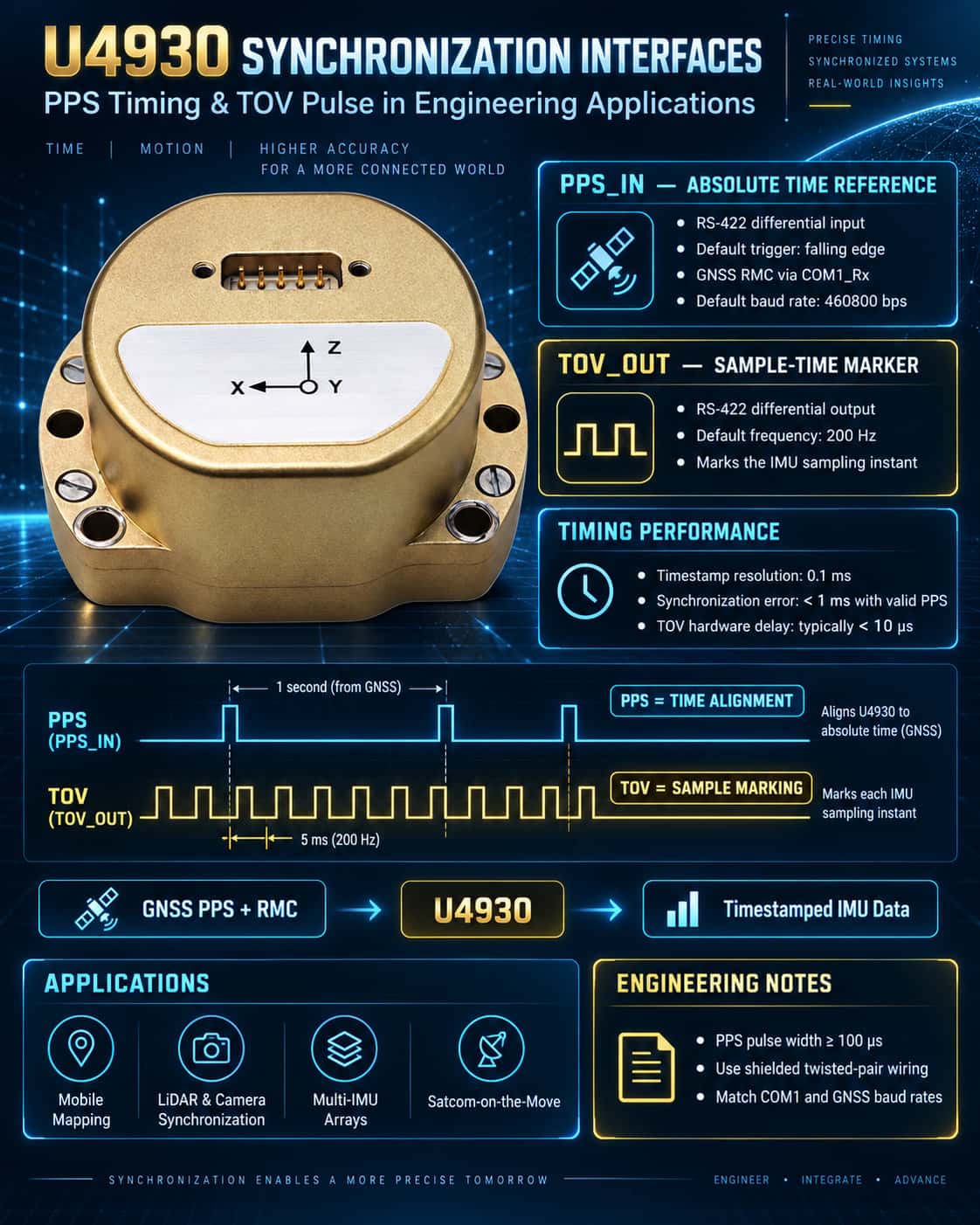
In integrated navigation systems, time synchronization is a critical factor determining data fusion accuracy. The U4930 MEMS IMU offers comprehensive synchronization interfaces—PPS input and TOV output—designed to handle the introduction of an external time reference and the calibration of internal sampling moments, respectively. Proper utilization of these interfaces significantly enhances system time-alignment accuracy, making the unit ideal for applications demanding strict clock consistency, such as UAV swarms, mobile mapping, and SATCOM-on-the-move (SOTM).   PPS_IN: The "Heartbeat" of the External Time Reference   PPS (Pulse Per Second) is a signal provided by Global Navigation Satellite Systems (GNSS); its rising or falling edge corresponds to the exact start of a second, typically with nanosecond-level precision. The U4930 receives the external PPS signal (RS-422 level) via the PPS_IN± differential interface while simultaneously receiving GPRMC/GNRMC/GBRMC sentences (default baud rate: 460800 bps) from the same GNSS source via the COM1_Rx± interface.   Internally, the system uses the PPS falling edge as the synchronization trigger (default configuration). Upon detecting a valid pulse, the IMU parses the UTC time from the most recently received RMC sentence on COM1 and aligns it with an internal counter, thereby generating a high-precision internal timestamp (Timestamp field, 0.1 ms resolution). This mechanism ensures that every data frame output by the IMU carries an absolute time tag consistent with the GNSS system, providing the necessary time reference for subsequent loose or tight coupling with GNSS position and velocity data.   Engineering Application Recommendations: · Ensure the PPS signal levels comply with the RS-422 differential standard to avoid latency introduced by single-ended conversion; · A PPS pulse width of ≥100 μs is recommended; the steepness of the falling edge directly impacts synchronization accuracy; · If the GNSS receiver outputs only a single-ended PPS signal, a differential converter is required to connect to the PPS_IN± interface; · The system supports configuration for either PPS rising-edge or falling-edge triggering; users can adjust this setting via the host computer based on the specific characteristics of the GNSS module. TOV_OUT: "Timestamp Marker" for Sampling Instants   TOV (Time of Validity) is a differential synchronization pulse signal (TOV±) actively output by the U4930; its frequency matches the IMU's internal sampling frequency (default: 200 Hz). The rising or falling edge of this pulse precisely corresponds to the start of the IMU data sampling interval, and its differential signal levels comply with the RS-422 standard.   The core value of TOV lies in enabling precise time-offset calculations between IMU sampling instants and external sensor acquisition times. When the U4930 operates alongside external devices (such as cameras, LiDAR, or scanners), these devices can capture the TOV pulse and record their local timestamps. By correlating this with the internal timestamp found in the IMU data frame, users can calculate the exact time lag and apply interpolation compensation during data post-processing or real-time sensor fusion.   Typical Application Scenarios: · Mobile Mapping Systems: Synchronizing the IMU with a laser scanner; TOV is used to calibrate the attitude timestamp corresponding to specific scan lines. · UAV Visual Navigation: TOV triggers camera exposure, achieving millisecond-level alignment between images and attitude data. · Multi-IMU Arrays: Synchronous acquisition of TOV signals from multiple U4930 units to achieve clock synchronization across multiple nodes.   Operational Mechanism and Engineering Considerations   (1) Relationship between PPS and TOV: PPS is used for "time synchronization," while TOV is used for "marking." Although they operate independently, using them in tandem enables precise tracing of sampling instants against a global time reference.   (2) Baud Rate Consistency: The default baud rate for GNSS input on COM1_Rx matches the IMU output baud rate (both are 460800 bps). If the output baud rate is changed, the GNSS module's baud rate must be updated accordingly; otherwise, RMC sentences cannot be parsed.   (3) Data Frame Timestamp Parsing: The Timestamp field in the protocol (bytes 35–38; conversion factor: 0.1 ms) represents an internal counter value. When PPS synchronization is active, this value is periodically corrected, resulting in an error of less than 1 ms. If no PPS signal is connected, the value relies on the internal crystal oscillator for timing, leading to cumulative drift. (4) TOV Latency Compensation: The TOV output entails an inherent hardware latency (typically <10 μs). If the system requires sub-microsecond synchronization, it is recommended to calibrate this latency value prior to factory shipment or to subtract the fixed offset during post-processing.   (5) ESD Protection and Wiring Reliability: Differential signal lines should utilize shielded twisted-pair cables and avoid running parallel to power lines to minimize common-mode interference.   In summary, the U4930’s PPS timing interface integrates the MEMS IMU into the GNSS absolute time framework, transforming it from a standalone "blind-reckoning" unit into a synchronization node within an integrated navigation system. Meanwhile, the TOV pulse provides a physical marker for sampling instants, facilitating timestamp alignment across multiple sensors. Together, these features enable the U4930 to achieve time synchronization accuracy superior to 1 ms in applications such as UAVs, autonomous driving, surveying and mapping, and COTM (Communications on the Move), thereby laying a solid foundation for highly reliable attitude determination and multi-source data fusion.

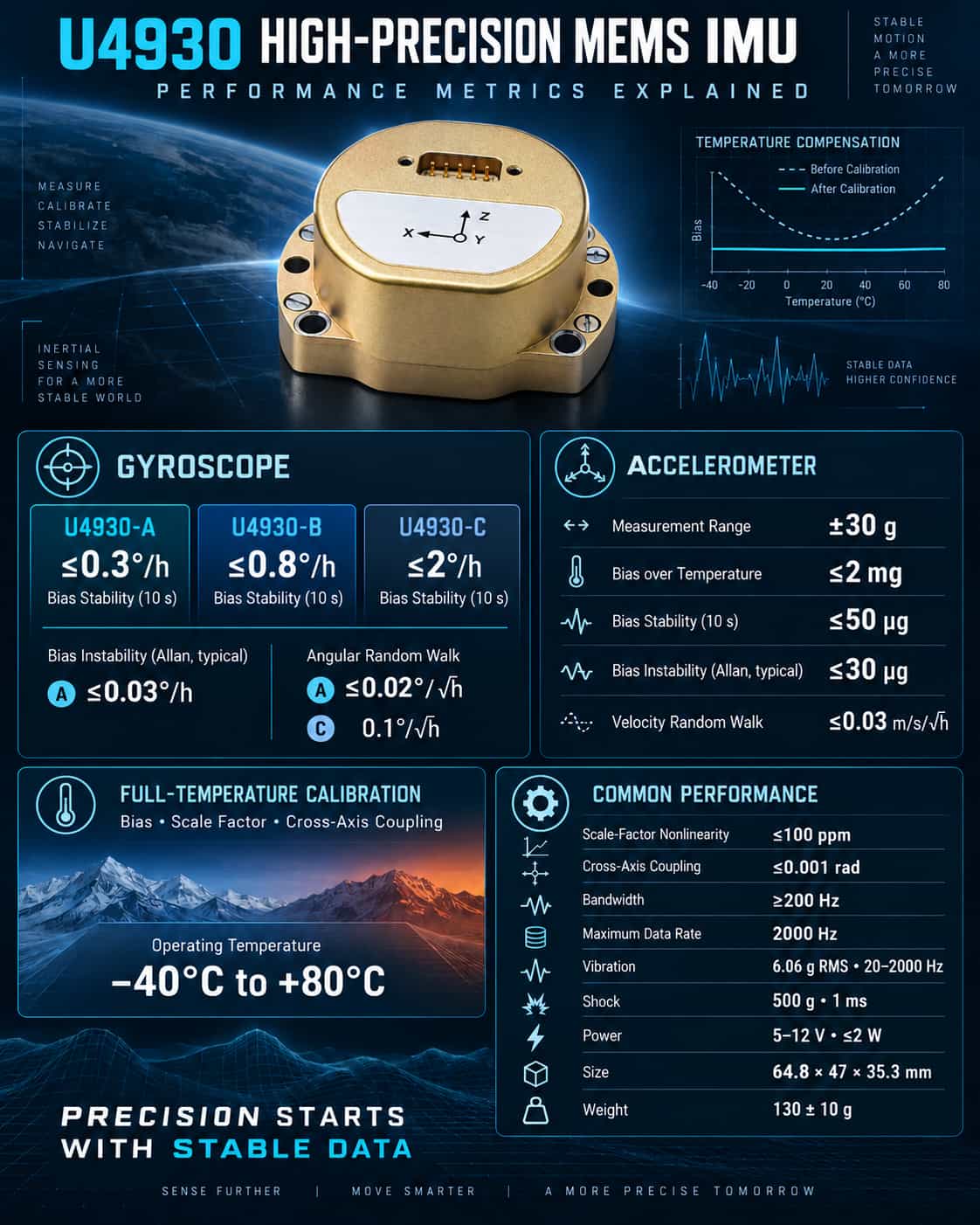
As the core sensing unit for inertial navigation and control, the performance parameters of an IMU directly determine the upper limits of accuracy for system attitude determination and navigation positioning. With distinct model classifications and full-temperature-range calibration capabilities, the U4930 series of MEMS IMUs offers performance options tailored to diverse application scenarios. This article provides a systematic analysis of the series' key performance indicators.   1. Gyroscope Performance: Precision Determines Attitude Stability   Gyroscope bias stability is a key metric for measuring long-term angular drift. The U4930-A model achieves ≤0.3°/h (10s), while the B model offers ≤0.8°/h and the C model ≤2°/h. For vessels or drones requiring sustained heading accuracy over long periods, the A model clearly holds the advantage; conversely, for cost-sensitive commercial vehicles where periodic recalibration is acceptable, the B or C models are sufficient.   Bias instability (characterized by Allan variance) reflects the ultimate noise floor. The A model’s typical value of ≤0.03°/h indicates minimal angular drift under ideal static conditions, making it suitable for high-precision surveying and track inspection.   Angle Random Walk (ARW) influences the accumulation of angular errors in dynamic environments. The A model’s ARW of ≤0.02°/√h is far superior to the C model’s 0.1°/√h, enabling better performance in flight control scenarios involving intense vibration or rapid maneuvering.   Notably, all three models feature scale factor nonlinearity of ≤100 ppm, cross-axis coupling of ≤0.001 rad, and a bandwidth of ≥200 Hz. These specifications ensure rapid response and minimal inter-axis interference, meeting the requirements of most real-time control applications.   2. Accelerometer Performance: Balancing Stability and Sensitivity   The entire U4930 series features an accelerometer measurement range of ±30g, covering the typical maneuvering ranges of vehicles, vessels, and drones. Key specifications include a full-temperature bias of ≤2 mg, bias stability of ≤50 μg (10s), bias instability of ≤30 μg (Allan typical value), and velocity random walk of ≤0.03 m/s/√h; these metrics place the series in the high-performance tier for MEMS-based sensors. For inertial navigation systems, accelerometer bias stability directly impacts the cumulative error in velocity and position calculations. A stability of 50 μg ensures that velocity errors remain at a low magnitude during one hour of pure inertial dead reckoning, making it suitable for navigation during brief GNSS signal outages.   3. Environmental Adaptability and Physical Characteristics   The entire U4930 series supports an operating temperature range of -40°C to +80°C and undergoes calibration across the full temperature range for bias, scale factor, and cross-coupling compensation. It demonstrates excellent mechanical robustness, with vibration tolerance of 6.06g (RMS, 20–2000 Hz) and shock tolerance of 500g/1ms. Key specifications include a supply voltage of 5–12V, steady-state power consumption ≤2W, startup time ≤2s, a maximum data rate of 2000 Hz, dimensions of 64.8 × 47 × 35.3 mm, and a weight of 130 ± 10 g, striking a balance between miniaturization and low power consumption.   4. Selection Recommendations and Summary   · U4930-A: Suitable for applications requiring extremely high performance regarding bias and random walk, such as mobile mapping, high-precision underwater navigation, and SATCOM-on-the-move (SOTM). · U4930-B: Suitable for medium-precision applications, such as UAV attitude reference, track inspection, and shipborne attitude measurement. · U4930-C: Suitable for cost-sensitive applications that tolerate higher drift, such as flight control and reference IMUs for commercial vehicles.   Overall, the U4930 series maximizes the potential of MEMS technology through full-temperature calibration and a modular design. When selecting a model, users should prioritize whether the gyroscope bias stability and angular random walk meet the system's long-term navigation accuracy requirements, while also evaluating bandwidth and shock resistance against environmental vibration conditions. Properly matching specifications with requirements ensures an optimal balance between performance and cost.

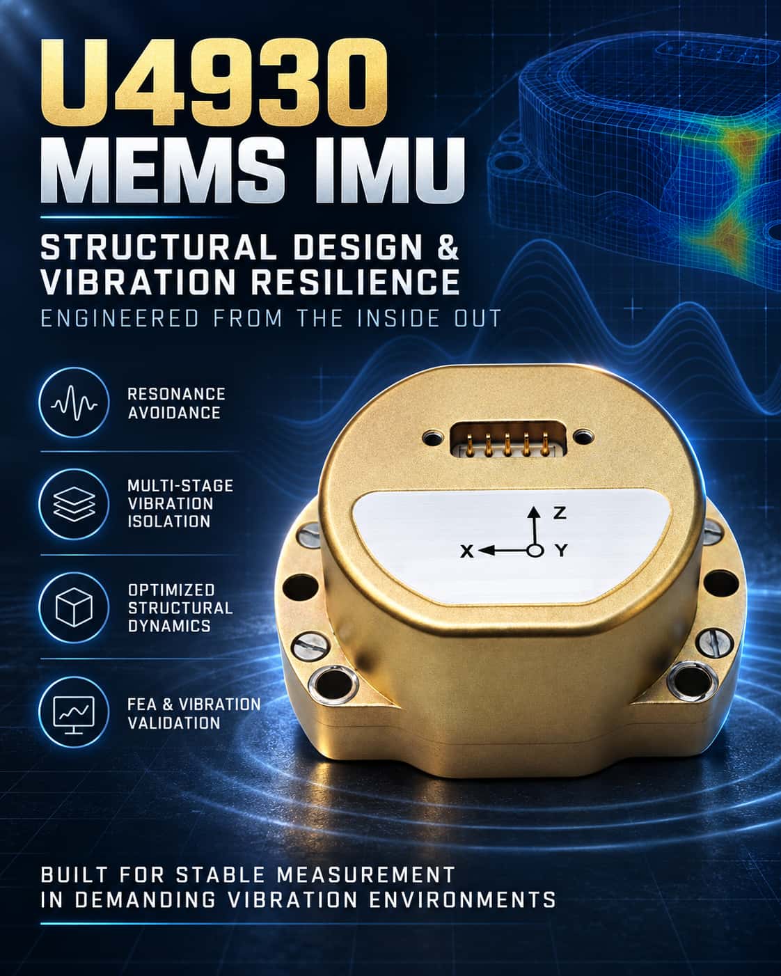
MEMS Inertial Measurement Units (MEMS IMUs) are widely used in fields such as navigation and attitude control; however, vibration environments can significantly degrade their measurement accuracy. Research indicates that external vibrations can cause severe output deviations in MEMS gyroscopes and may even lead to structural fatigue or fracture. Consequently, employing rational structural design and vibration-resistance optimization at the system level is crucial for enhancing the environmental adaptability of MEMS IMUs.   **Vibration Interference Mechanisms and Design Objectives**   The fundamental reason for the vibration sensitivity of MEMS IMUs lies in their operating principles. Taking the gyroscope as an example, its operation relies on the coupling between drive and sense modes; if external vibrations couple into these modes, they directly translate into output errors. Furthermore, structural resonance induced by vibration amplifies this effect. Therefore, structural design pursues two core objectives: first, avoiding resonance by using modal analysis to ensure the structure's natural frequencies remain well away from the frequency bands where vibration energy is concentrated; and second, isolating vibration by incorporating vibration-isolation elements along the transmission path to attenuate the vibration energy reaching sensitive components.   **Key Structural Design Strategies**   Current structural design approaches primarily follow two technical paths:   First, system-level vibration isolation structures. Vibration isolation systems are created by embedding isolators (such as rubber pads or metal springs) between the IMU and the host platform, or between the internal core and the outer housing. Research suggests that to meet the compact size requirements of MEMS IMUs, multi-stage isolation designs can be employed—such as arranging three levels of damping pads (housing–core–measurement assembly) and utilizing stiffness gradients to achieve staged attenuation. More advanced solutions utilize motion-decoupling mechanisms to design six-degree-of-freedom isolation systems, thereby suppressing vibration coupling effects caused by isolator asymmetry. In typical applications, the use of a two-stage lattice isolation structure combined with redundant, multi-sensor 3D mounting can reduce the root-mean-square (RMS) value of angular velocity output by more than 88% under flight vibration spectra.   Second, optimization of sensitive structures. At the chip level, vibration resistance can be enhanced at the source by employing high-symmetry structural designs (such as eight-mass or ring structures) that utilize differential principles to cancel out common-mode vibration interference, or by using a single-mass tri-axial gyroscope design featuring a central anchor and symmetric flexure bearings.   Design Verification and Performance Evaluation   Finite element analysis (FEA) serves as the most critical verification tool in this field. Modal analysis allows for the calculation of natural frequencies to assess resonance risks, while frequency response and random vibration analyses predict acceleration responses under specific power spectral densities, providing a basis for design iteration. Experimental verification typically encompasses calibration and vibration testing. For instance, one optimized design—utilizing methods such as adding support beams and reducing fixed spans—more than doubled the vibration resistance of the IMU compared to the original design; another lightweight IMU demonstrated excellent vibration resistance alongside high precision during vibration testing.   In summary, the vibration resistance of MEMS IMUs is a system-level issue that requires a structural dynamics perspective and the integrated application of techniques such as modal analysis, vibration isolation design, and optimization simulation. Adopting "avoiding resonance" and "efficient vibration isolation" as core design principles offers an effective pathway for developing highly reliable MEMS IMUs. Looking ahead, advancements in materials science and control algorithms will enable MEMS IMUs to maintain performance in increasingly extreme vibration environments, opening up broader application prospects.

Core Application: Guidance and Attitude Control   The G-F3G70 tri-axial fiber optic gyroscope (FOG) is specifically designed for medium-to-high precision navigation, guidance, and attitude control systems. It serves as a critical sensing core enabling precision strikes and flight control for tactical weapons such as small missiles and guided bombs. By integrating angular rate sensing capabilities across three axes, it accurately detects the carrier's 3D attitude changes and angular motion in real-time. It provides vital data to the flight control computer, ensuring the weapon platform maintains stable flight along its intended trajectory and strikes the target with precision.   Technical Advantages: High Precision and High Reliability   As an all-solid-state gyroscope, the G-F3G70 inherits the inherent advantages of fiber optic gyroscopes: rapid startup, wide dynamic range, and high reliability. Its superior performance fully meets the requirements of navigation and guidance-grade applications: · Excellent Bias Stability: The G-F3G70-C model achieves bias stability of ≤0.02°/h (10s smoothing), ensuring an accurate and stable attitude reference during long-duration flight missions. · High Dynamics and Sensitive Response: The product features a dynamic measurement range of ±300°/s and a bandwidth of ≥200Hz, enabling precise tracking of attitude changes during high-speed, high-maneuverability flight. Additionally, a threshold and resolution of ≤0.01°/h ensure the system's keen sensitivity to minute angular movements. · Harsh Environment Adaptability: It supports an operating temperature range of -45°C to +65°C and features a lightweight design (under 800g). Combined with the FOG's inherent shock and vibration resistance, it is ideally suited for demanding environments such as missile-borne applications.   Ease of System Integration   The G-F3G70 utilizes an integrated optical-electronic packaging design with a split-unit structure, resulting in a compact form factor and easy installation. The electronics module measures 60×60×24mm, while the sensor head measures Φ67mm×17.5mm. It includes clearly defined M3×4 and Φ2.7×8 mounting holes, facilitating integration into space-constrained weapon systems. The product operates on a standard +5V power supply with a steady-state power consumption of ≤5.5W, and outputs digitized angular rate and temperature data via a high-speed serial port (921600 bps, even parity), greatly simplifying the user's electrical and communication interface design.

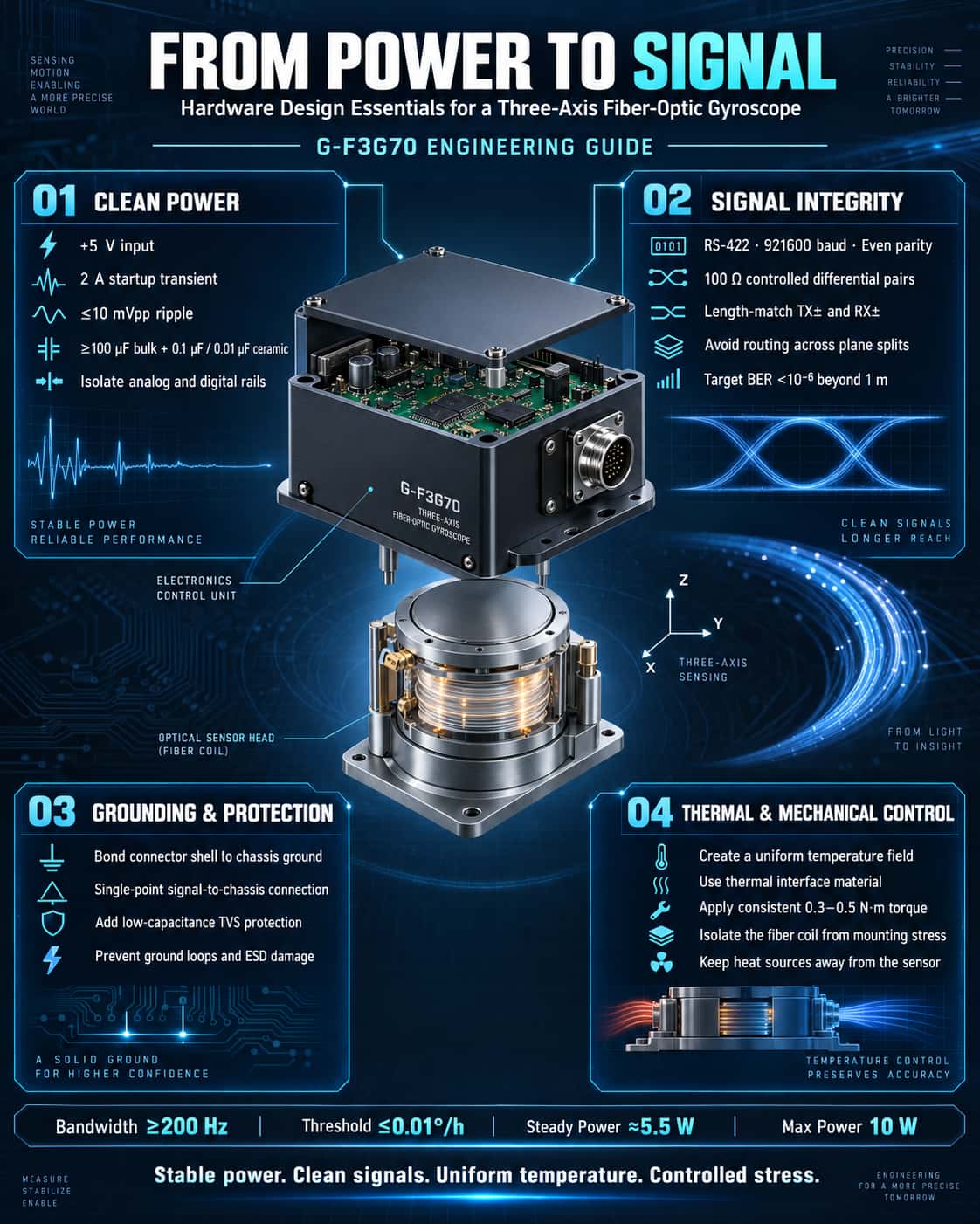
Thanks to advantages such as solid-state construction, rapid startup, wide dynamic range, and high reliability, three-axis fiber-optic gyroscopes (FOGs) play a critical role in small missiles, guided bombs, and high-precision attitude control systems. However, fully realizing their performance potential requires meticulous attention to hardware design—particularly regarding power supply, signal chains, and interface layout. Using the G-F3G70 three-axis FOG as a case study, this article outlines key design considerations from an engineering perspective.   1. Power Supply Design: Low Noise and Transient Response as Primary Considerations   A gyroscope's bias stability and angle random walk (ARW) coefficient are directly affected by power supply quality. The G-F3G70 requires a +5V power supply; the instantaneous startup current can reach 2A, while steady-state power consumption is approximately 5.5W (peaking at 10W across the full temperature range). Design efforts should focus on the following: · Low-noise LDOs or post-stage DC-DC filtering: Switching ripple must be controlled to within 10mVpp—especially in the 100Hz to 1MHz frequency range—to prevent coupling into the signal processing chain and degrading the angle random walk performance. · Adequate decoupling capacitance: High-capacity tantalum capacitors (≥100μF) combined with high-frequency ceramic capacitors (0.1μF and 0.01μF in parallel) should be placed at the connector inputs (pins 5 and 13 of the J30-15ZKP). This ensures the system can handle the 2A startup current surge and prevents voltage drops that could trigger resets or data anomalies. · Power and ground plane isolation: A single-point connection—using a ferrite bead or a low-value resistor—is recommended between the digital power supply (interface side) and the analog power supply (internal gyroscope conditioning circuitry). This prevents digital noise from radiating through the power lines and interfering with sensitive optoelectronic detection components.   2. Signal Interface: Differential Transmission and Robust Grounding   The G-F3G70 utilizes an RS-422 serial interface with a baud rate of 921,600 and even parity. The data output includes three-axis angular rates (32-bit signed integers) and three temperature readings (16-bit signed integers with 1/16 resolution). Hardware design guidelines: · Strict differential pair length matching: TX+/TX- and RX+/RX- signals must be routed as differential pairs with controlled impedance (typically 100Ω). Avoid routing across split planes to suppress common-mode interference and ensure a bit error rate (BER) of less than 10⁻⁶ for long-distance (>1m) transmission. · Shielding and grounding: The connector housing should be connected to chassis ground (PE), while signal ground (GND) connects to PE at a single point via an RC parallel network (e.g., 10Ω + 0.1μF). This prevents ground loops from introducing power-frequency interference that could compromise bias repeatability (specification: ≤0.03–0.05°/h). · ESD protection: TVS diodes (e.g., SMCJ5.0CA) must be installed on all interface pins (especially R+/R-) to prevent damage to the internal RS-422 driver chips caused by hot-plugging or electrostatic discharge.   3. Mechanical structure and thermal management: Temperature gradients determine bias stability   The G-F3G70 exhibits a bias stability of 0.10–0.15°/h under varying temperature conditions (1°C/min), indicating that temperature gradients are the primary source of error. Engineering best practices include: · Thermal conduction at the mounting interface: Both the circuit housing (60×60×24mm) and the sensor head (Φ67×17.5mm) must make tight contact with the mounting structure. Applying thermal grease is recommended to reduce thermal resistance and ensure a uniform temperature field across the unit, thereby preventing localized hot spots from causing refractive index changes in the fiber optic coil. · Stress isolation: Fastening torque for mounting holes (M3×4 and Φ2.7×8) must be consistent (recommended: 0.3–0.5 N·m). Excessive mechanical stress transmitted through the housing to the fiber optic coil can induce birefringence, leading to increased bias drift. The use of flexible washers or O-rings is recommended for stress isolation. 4. Layout and Connector Selection: Defining Signal Flow   The pin assignments for the J30-15ZKP connector clearly define the power supply (red/black) and serial port (yellow/orange/blue/green) connections. Key layout considerations include: · High/Low-Voltage Separation: Route the +5V power line (red) and signal lines (yellow/blue) on separate PCB layers or with adequate spacing (≥3W, where W is the trace width) to minimize interference from the power supply's magnetic field on the differential signals. · Temperature Sensor Routing: While the three temperature channels (internal signals output as data) require no external processing, users performing calibration must ensure that no heat sources (such as high-power resistors) directly radiate heat onto the gyroscope body; otherwise, deviations between temperature readings and the actual ambient temperature will compromise the accuracy of the compensation model.     In summary, the hardware design of a three-axis fiber-optic gyroscope involves far more than simply connecting power and reading serial data. From power supply transient response and differential signal integrity to thermal management and mechanical stress relief, every aspect is closely linked to core performance metrics such as bias stability, repeatability, and random walk. By adhering to these guidelines and utilizing the detailed specifications from the G-F3G70 manual (e.g., bandwidth ≥200 Hz, threshold ≤0.01°/h), the system can reliably achieve navigation-grade angular rate measurement under actual operating conditions, providing a dependable data foundation for high-dynamic control applications.

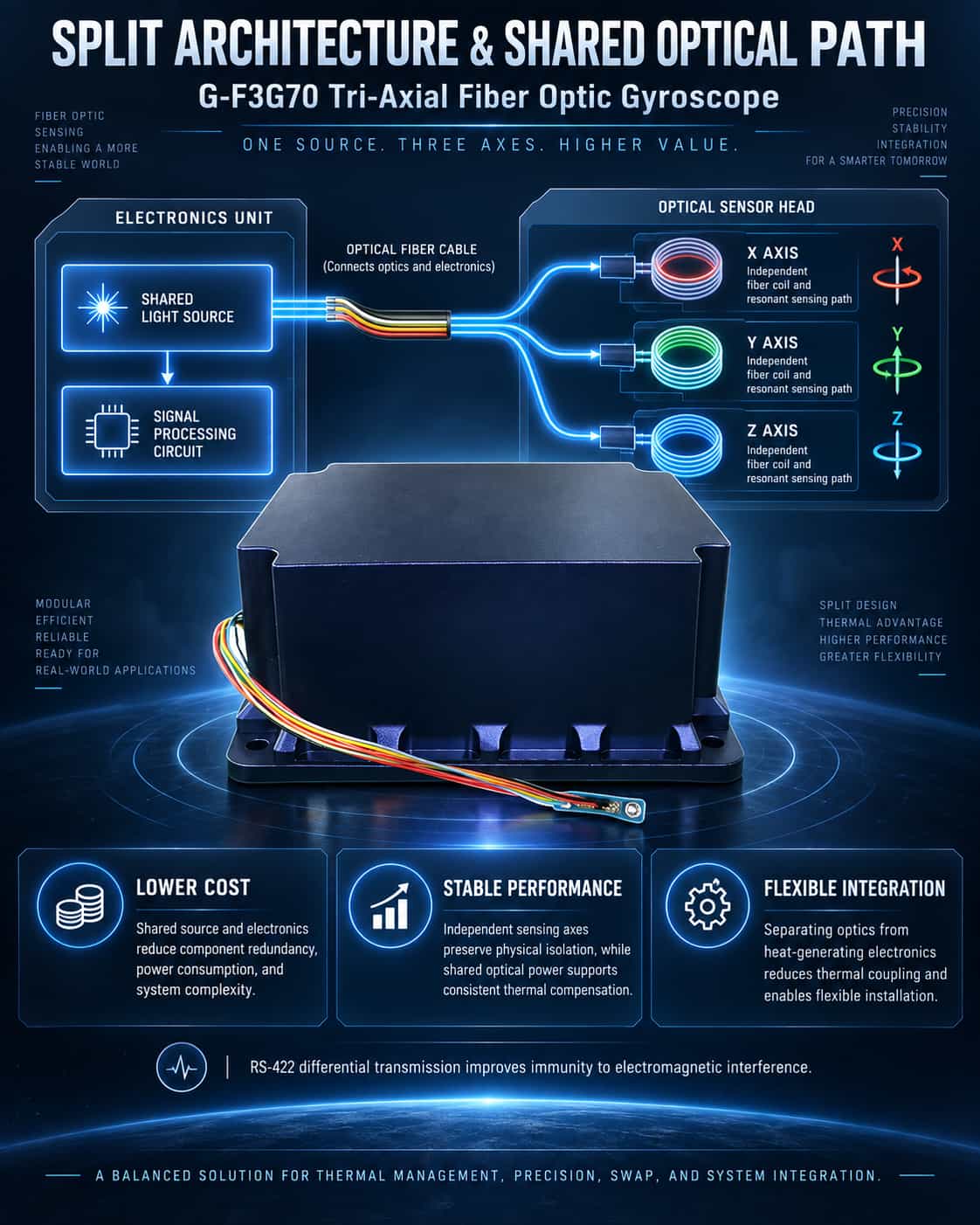
The core technical requirement for a tri-axial fiber optic gyroscope (FOG) is to integrate three sensing axes—measuring angular rates along the X, Y, and Z axes respectively—within the smallest possible volume, while ensuring that the three axes remain independent and free from mutual interference.   The G-F3G70 tri-axial FOG employs a technical approach where the light source and signal processing circuitry are shared across all three axes, yet each axis retains its own independent fiber coil and resonant cavity. In simpler terms: while the light source and circuitry are shared, the sensing core for each axis remains independent. The primary advantages of this approach include a reduction in redundant components, lower overall power consumption and cost, and the elimination of cross-interference between three separate sets of circuits. Furthermore, sharing a single light source ensures consistent optical power across all three axes, facilitating unified modeling for temperature compensation algorithms.   Split Architecture: Separation of Circuitry and Optics   The most distinct structural feature of the G-F3G70 is the separation of the electronics unit and the sensor head, connected by a cable. What is the engineering rationale behind this split design?   The core components of a fiber optic gyroscope—such as the light source, detector, modulator, and fiber coil—are optical devices that are extremely sensitive to temperature fluctuations and mechanical stress. In contrast, the electronics section, which handles signal processing, power management, and communication interfaces, generates heat during operation.   If optical components and circuitry were tightly packaged within the same housing, heat generated by the electronics would transfer directly to the fiber coil. This would create localized temperature gradients, leading to thermally induced non-reciprocity errors—one of the primary sources of error in fiber optic gyroscopes. The split design physically separates the heat source (electronics) from the sensitive elements (optical components), fundamentally reducing thermal coupling effects.   Additionally, the split design offers greater flexibility for system integration. The electronics unit and the sensor head can be mounted in different locations on the host platform: the sensor head can be placed near the platform's center of gravity for precise angular motion sensing, while the electronics unit can be situated in an area with more space or better heat dissipation. Connected by a flexible cable, the two units do not restrict each other's mounting position or orientation.   Engineering Trade-offs and Compensation for the Split Design   The split design does not come without a cost. When the circuitry is separated from the sensor, the weak signals carried by the cables become susceptible to electromagnetic interference; consequently, the G-F3G70 employs RS-422 differential signaling for external communication, ensuring high common-mode rejection and robust interference immunity. Furthermore, signal pre-amplification and filtering are performed within the sensor head, guaranteeing that the output signal possesses an adequate signal-to-noise ratio.   In addition, the split design imposes stricter requirements on installation precision. The mounting surface of the electronics unit and the locating shoulder of the sensor head must be accurately aligned with the carrier's reference datum; any angular misalignment translates directly into non-orthogonality errors between the three axes, thereby compromising north-finding accuracy and navigation solution results.   Summary of Design Logic   The core design logic behind the G-F3G70’s architecture—featuring a shared optical path for three axes combined with a split-unit structure—can be summarized as follows:   ` Shared light source and circuitry across three axes—reduces power consumption, cost, and complexity while ensuring axis-to-axis consistency; ` Independent sensing axes—maintains physical independence of the three-axis sensing function, preventing motion coupling and signal crosstalk; ` Physical separation of optics and electronics—isolates heat sources and protects optical components from thermal and mechanical stresses; ` Split-unit installation for enhanced flexibility—accommodates the spatial constraints of various carriers and simplifies system integration.   Overall, this design is not merely for aesthetics but addresses two fundamental contradictions in the engineering of fiber-optic gyroscopes: the trade-off between thermal management and accuracy, and the conflict between component size and installation flexibility. By adopting a split-unit architecture as an optimal engineering compromise, the G-F3G70 delivers medium-to-high precision performance while meeting the comprehensive requirements for size, weight, power consumption, and reliability demanded by tactical-grade navigation and guidance systems.

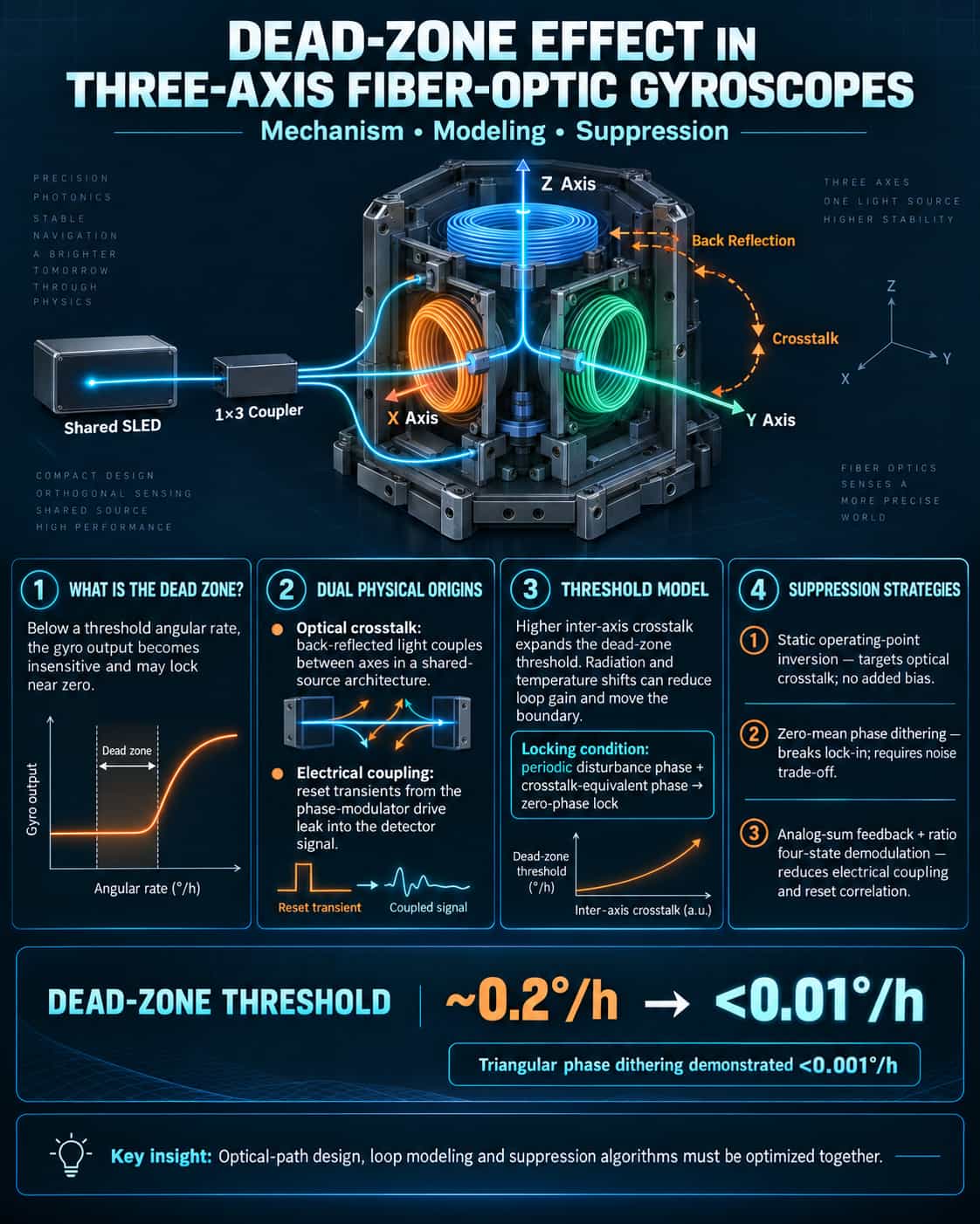
As three-axis fiber-optic gyroscopes (FOGs) increasingly aim for miniaturization and high precision, the "dead-zone" effect—triggered by inter-axis optical crosstalk—has become a critical bottleneck limiting performance in low-angular-rate measurements. A dead zone occurs when the gyroscope's output ceases to respond to changes in input angular velocity below a certain threshold. For applications such as satellite attitude control that require operation near zero angular velocity, the nonlinear bias error introduced by the dead zone directly compromises system accuracy. This paper focuses on the issue of inter-axis optical crosstalk in three-axis FOGs utilizing a shared-light-source architecture; it analyzes the underlying physical mechanisms, quantifies the impact on threshold characteristics, and comparatively evaluates current primary mitigation strategies.   **Physical Origins of the Dead Zone and the Inter-Axis Optical Crosstalk Model**   The dead zone is a nonlinear effect characteristic of digital closed-loop FOGs. Conventionally, the primary source of interference causing the dead zone is identified as the electrical cross-coupling of the staircase voltage applied to the phase modulator into the detector signal. However, in a three-axis shared-source architecture, the problem is more complex: a single superluminescent diode (SLD) source drives three orthogonal axes simultaneously after being split by a 1×3 coupler. Back-reflected light creates optical crosstalk channels between the axes; at low angular rates, this optical intensity crosstalk superimposes onto the interference intensity, potentially overwhelming the useful signal.   To quantitatively characterize this effect, a study proposed an open-loop excitation method to measure the optical back-reflection crosstalk coefficients between axes. Incorporating these coefficients into a closed-loop control model reveals that an increase in the crosstalk coefficient causes the gyroscope's threshold to expand multiplicatively, directly resulting in a wider dead-zone range. This mechanism can be formalized as follows: when the phase of the periodic disturbance in the feedback channel and the equivalent phase of the crosstalk satisfy specific conditions, the system enters the dead zone, and the output phase locks to zero.   **Quantitative Characterization of Dead-Zone Thresholds**   The impact of the dead zone on the system lies not only in the existence of an "insensitive range" but also in the fact that the boundaries of this range shift dynamically due to environmental factors such as space radiation and temperature fluctuations. Space radiation causes a decrease in light source power and an increase in fiber loss, thereby reducing the system gain (K₁) and expanding the dead-zone range. Experimental data indicate that the dead-zone threshold of an uncompensated triaxial gyroscope can reach the order of 0.2°/h, a level unacceptable for high-precision applications requiring the resolution of extremely low angular velocities.   It is worth noting that the dead zone arises from multiple mechanisms. In addition to inter-axis optical crosstalk, electrical cross-coupling constitutes another significant cause. The analog drive voltage signal of the phase modulator—subjected to resets via a digital feedback staircase wave—generates distinct operating modes; the resulting crosstalk, manifesting as variations in the amplitude and phase of the detector output signal, becomes particularly pronounced during state transitions in the four-state modulation scheme. Since these two mechanisms often act concurrently in triaxial systems, modeling the dead zone requires accounting for both optical and electrical dimensions.   Comparative Analysis of Suppression Schemes   To address the aforementioned causes of dead zones, three primary suppression strategies have been developed, each differing in mechanism and effectiveness:    Static operating point flipping (bias switching) method. Targeting the physical root cause of inter-axis optical crosstalk, this method actively flips the gyroscope's static operating point so that the crosstalk signal no longer superimposes onto the closed-loop residual phase. Experimental results are impressive: this approach reduces the threshold from 0.2°/h to below 0.01°/h, effectively enhancing measurement accuracy at low rotation rates. Its advantage lies in directly addressing the optical crosstalk mechanism without introducing additional bias errors.    Periodic perturbation superposition method (dithering). A zero-mean periodic perturbation phase, φ₀, is introduced into the system to break the dead-zone locking condition through "dithering." When the dither amplitude is sufficiently large (φ₀ ≥ φ₁), the dead zone can be completely eliminated. In practical engineering applications, triangular-wave phase dithering technology has suppressed the dead-zone error of high-precision gyroscopes from 0.08°/h to below 0.001°/h. The method's effectiveness has been validated in a triaxial system utilizing 900 meters of optical fiber; suppression performance depends on the specific combination of dither amplitude, frequency, and loop gain. However, excessive dither amplitude may introduce additional noise, necessitating a careful trade-off.    Combined method of analog additive feedback and ratio-based four-state demodulation. This method addresses the issue starting with the electrical cross-coupling path: in traditional four-state modulation, the reset operations associated with each modulation state are a primary cause of the dead zone. The analog additive feedback method significantly reduces the frequency of reset operations by resetting only the feedback phase during modulation; experiments demonstrate that this can lower the dead zone to below the measurement threshold of 0.022°/h. However, due to the inherent nature of electrical crosstalk, this method still introduces an additional bias of approximately -0.06°/h. To mitigate this, the method is further combined with the ratio-based four-state demodulation technique; by adjusting the demodulation ratio of the feedback signal, the correlation between the modulation and demodulation sequences is weakened, thereby controlling the additional bias while simultaneously suppressing the dead zone.   Overall, these three types of schemes are suited to different application scenarios: the optical crosstalk suppression scheme is most effective for tri-axial architectures sharing a common light source; the dithering method is simple to implement but requires noise management; and electrical crosstalk suppression schemes are better suited for single-axis and discrete systems. For silicon-photonic gyroscopes aiming for ultra-high integration, recent research has introduced a joint suppression algorithm that integrates phase-shift hopping with sample rejection; this approach suppresses the dead zone while reducing angle random walk by over 26%, reflecting a trend toward combining multiple strategies rather than relying on a single method.   In summary, the dead zone effect in tri-axial fiber-optic gyroscopes is a systemic issue resulting from the coupling of multiple factors. Inter-axis optical crosstalk and electrical cross-coupling constitute the physical root causes of the dead zone, with their effects significantly amplified in architectures featuring common light sources and high levels of integration. Currently, the static operating point bias-flipping method offers the best performance for optical crosstalk suppression, the dithering method boasts the broadest applicability, and combined modulation schemes represent the cutting edge of electrical crosstalk suppression. As tri-axial gyroscopes evolve toward chip-scale integration, the combination of inter-waveguide crosstalk suppression (e.g., germanium-doped silica waveguide chips achieving crosstalk levels below -40 dB) and algorithmic joint suppression strategies may well become the key pathway to completely resolving the dead zone problem.

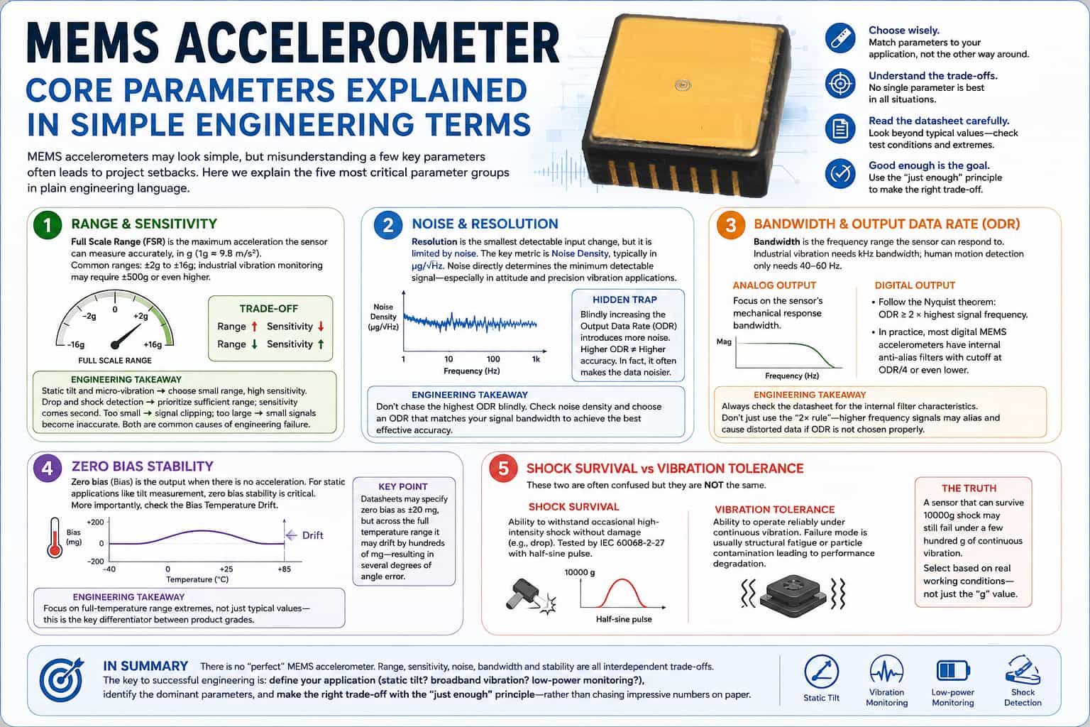
While MEMS accelerometers may appear simple during the engineering selection process, misunderstandings regarding a few core parameters often lead to costly setbacks. The following section explains the five most critical sets of parameters using engineering terminology, avoiding overly abstract theory.   **Full-Scale Range and Sensitivity**   Full-scale range refers to the maximum acceleration a sensor can accurately measure, typically expressed in *g* (where 1*g* ≈ 9.8 m/s²). Standard applications usually range from ±2*g* to ±16*g*, whereas industrial vibration monitoring may require ±500*g* or higher. Range and sensitivity are generally inversely proportional; a higher range comes at the cost of sensitivity to small signals. The selection logic is straightforward: choose a low range and high sensitivity for static tilt measurement or micro-vibration monitoring; conversely, prioritize sufficient range for drop or shock detection, where sensitivity is a secondary concern. Selecting a range that is too low leads to signal clipping, while one that is too high results in poor accuracy for small signals—both scenarios are common causes of engineering failure.   **Noise and Resolution**   Resolution represents the smallest input change a sensor can distinguish, yet it is constrained by noise. The key metric here is noise spectral density, typically measured in µg/√Hz. Noise directly determines the minimum detectable signal; in applications such as attitude sensing and precision vibration monitoring, noise levels warrant greater attention than resolution. A common engineering pitfall is the blind increase of the Output Data Rate (ODR), which introduces more noise. Many developers push the ODR to its maximum, only to find the resulting data riddled with noise; the root cause is that higher sampling rates often degrade effective precision.   **Bandwidth and Output Data Rate (ODR)**   Bandwidth defines the frequency range of input signals to which the sensor can respond. Industrial vibration monitoring requires a bandwidth of several kilohertz, whereas 40–60 Hz suffices for human motion tracking. For analog outputs, the focus is on the sensor's mechanical response bandwidth; for digital outputs, the Nyquist sampling theorem applies—meaning the ODR must be at least twice the highest signal frequency. A more subtle issue in practical engineering is that the internal anti-aliasing filter cutoff frequency for most digital MEMS accelerometers is only one-quarter (or less) of the ODR. If the ODR is selected based solely on the "2x" rule during mechanical design, high-frequency signal aliasing will directly result in data distortion. Always consult the filter characteristics in the datasheet rather than relying on theoretical formulas.   Bias Stability   Bias refers to the output value when no acceleration is present. For static applications such as tilt detection, bias stability is of paramount importance. Even more critical is bias temperature drift. Some devices may specify a bias of ±20 mg in their datasheets, yet drift by hundreds of milligrams across the full temperature range—an error that translates into a deviation of several degrees in angle. This is a key differentiator between product grades; one must focus on extreme values ​​across the full temperature range rather than typical values.   Shock Limit vs. Vibration Tolerance   These parameters are easily confused. Shock resistance refers to the ability to withstand occasional, high-intensity impacts (such as drops) without damage; the testing standard is IEC 60068-2-27, utilizing a half-sine pulse. Vibration tolerance, conversely, concerns the ability to operate reliably over the long term under continuous vibration, where failure modes include structural fatigue or performance degradation caused by particulate contamination.   The two are not interchangeable; a sensor capable of withstanding a 10,000g shock might fail under continuous vibration of only a few hundred g. Selection must be based on the actual operating environment rather than simply prioritizing the highest "g-rating."   In summary, there is no "universal parameter" for selecting MEMS accelerometers; the factors of range, sensitivity, noise, bandwidth, and stability involve inherent trade-offs. Successful engineering implementation relies on clearly defining the application scenario (e.g., static tilt, broadband vibration, or low-power monitoring), identifying the dominant parameters, and making choices based on the principle of "sufficiency" rather than chasing impressive specifications on paper.