
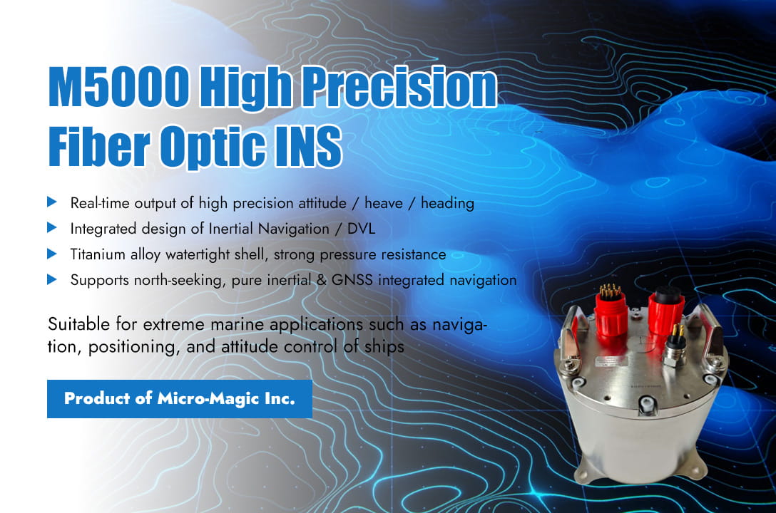
One-minute quick read The Fiber Optical Strapdown Inertial Navigation System (FOG-SINS) uses fiber optic gyroscopes (FOGs) and accelerometers to form a solid-state inertial measurement unit (IMU), which calculates the motion parameters of the carrier in real time through a strapdown algorithm. Due to its significant technological advantages, FOG-SINS has become the core of the new generation of navigation systems in the field of ocean ships. The application of FOG-SINS in the field of ocean ships is mainly reflected in ship navigation, underwater vehicle control, and multi beam measurement. Its core advantages are high precision, high reliability, strong anti-interference ability, autonomous navigation, excellent dynamic performance, and good environmental adaptability. Ship Navigation FOG-SINS can provide continuous and autonomous ship position, heading, attitude (roll, pitch), velocity, and acceleration information for navigation. FOG-SINS is integrated with GNSS (GPS, Beidou, etc.), odometry (Doppler/electromagnetic), compass (magnetic/electric compass), etc. (usually through Kalman filtering) to form a high-precision and high reliability integrated navigation system. FOG SINS provides critical navigation capabilities in the event of GNSS signal interference, obstruction, or failure (such as in canyons, under bridges, electronic warfare environments). FOG-SINS can also provides high-precision attitude reference information for shipborne weapon. The Technical Advantages of FOG-SINS in Ship Navigation : ⚪ High precision and stability: The zero bias stability of modern high-precision FOGs can reach the order of 0.01°/h or even higher, and the angle random walk can reach the order of 0.001°/√h, which can support long-term, high-precision inertial navigation requirements and significantly reduce the accumulation speed of position errors. ⚪ Quick start and response, wide dynamic range: Short start time (much shorter preheating time than mechanical gyroscopes), fast dynamic response, and accurate capture of the ship's rapid maneuvering (such as emergency steering and collision avoidance). Capable of measuring various ship movements from extremely low to high speeds. ⚪ Strong environmental adaptability and resistance to impact and vibration: relatively insensitive to changes in marine environmental factors such as temperature, humidity, and salt spray (especially after good design and compensation), with high reliability. The all solid state structure (without mechanical rotating parts) provides strong immunity to the inherent impacts and vibrations during ship operation, with stable performance and long lifespan. Underwater Vehicle (AUV/UUV) Control FOG SINS, as the core component of the underwater submersible control system, is the core sensor for AUVs to achieve long-term and high-precision autonomous navigation in the absence of GNSS signals underwater. Provide position, attitude, velocity, and acceleration information. The combination of FOG SINS, Doppler log (DVL), depth meter, magnetometer (heading assist), ultra short baseline/long baseline acoustic positioning system (USBL/LBL), gravity/geomagnetic matching navigation, etc., forms an underwater integrated navigation system, greatly improving navigation accuracy and reliability. FOG SINS is the core and foundation of integrated navigation. FOG SINS provides high-precision real-time attitude and heading feedback for the control system of AUVs (such as rudder, thruster, attitude adjustment mechanism), achieving precise depth, height, directional navigation, and complex maneuvers (such as hovering and bottom mounted navigation). Provide a stable attitude reference for task payloads such as sonar (side scan, front view), cameras, and robotic arms to ensure data quality and operational accuracy. The Technical Advantages of FOG SINS in Underwater Submersible Control System : ⚪ Complete autonomy: not relying on external signals, is the key to achieving true autonomous navigation underwater. ⚪ High precision (especially important underwater): High precision attitude and heading information is crucial for underwater obstacle avoidance, terrain tracking, and precise operations. Good zero bias stability can prolong the pure inertial navigation time underwater. ⚪ Anti magnetic field interference: Fiber optic gyroscopes are based on optical principles and are not affected by the complex magnetic field environment underwater (while magnetic compasses are affected). Multi Beam Measurement System The FOG SINS can provide motion compensation for multi beam measurement systems, which is the most core application of FOG SINS in multi beam depth measurement. Accurately measure and compensate in real-time for the attitude changes (roll, pitch, yaw) and heave movements of the measuring vessel/platform at the moment of measurement. FOG SINS can provide accurate heading angle and position information for multi beam measurement system (usually tightly coupled with GNSS), used to determine the precise position and direction of sonar array in the geodetic coordinate system. FOG SINS can provide accurate time reference for the entire measurement system (multibeam sonar, GNSS, motion sensors, sound speed profiler, etc.). The Technical Advantages of FOG SINS in Multi Beam Measurement System: ⚪ Ultra high dynamic performance and bandwidth: capable of accurately and quickly measuring and responding to high-frequency movements of ships/platforms (especially heave and sway caused by short period waves), which is the key to obtaining high-quality seabed terrain data. Its dynamic response capability far exceeds traditional vertical reference units (VRUs). ⚪ High attitude accuracy: The accuracy of attitude (especially roll and pitch) directly affects the compensation accuracy of beam angle. FOG SINS can provide sub angular (<0.01 °) level attitude measurement accuracy, ensuring the accuracy of beam pointing and seabed footprint position calculation. ⚪ Tight integration and time synchronization: FOG SINS are typically designed as highly integrated measurement units (often referred to as POS MV or INS), with internal sensors (gyroscopes, accelerometers) having extremely high synchronization accuracy and the ability to achieve microsecond level time synchronization with other external sensors (GNSS, sonar), ensuring strict alignment of all data in time. Key Products & Technical Specifications Parameter IF3600 IF3700 Pure inertial alignment accuracy North finding accuracy ≤0.1°sec(Φ) ≤0.05°sec(Φ) Attitude accuracy ≤0.008° ≤0.003° Pure inertia retention accuracy Heading angle 0.03°/h ≤0.01° Attitude angle 0.02°/h ≤0.005° Position(CEP50%) ≤1 nmile/h ≤1nmile/h velocity ≤0.5m/s ≤0.5m/s Inertial/satellite combination accuracy Heading ≤0.02° ≤0.02° Attitude ≤0.005° ≤0.005° Position ≤ 2m (单点) ≤ 2cm+1ppm(RTK) ≤1.2m (单点) ≤2cm+1ppm(RTK) Velocity ≤0.02m/s ≤0.02m/s Inertia/ODO/DVL combination accuracy Milemeter/DVL combination 0.25% ×D ≤0.5%×D Conclusion Fiber optic strapdown inertial navigation system has become an indispensable core technology in modern ship high-precision navigation, autonomous operation of underwater vehicles, and high-resolution seabed terrain mapping due to its advantages of all solid state high reliability, dynamic accuracy, and multi-sensor fusion capability. M5000 M1000
Read More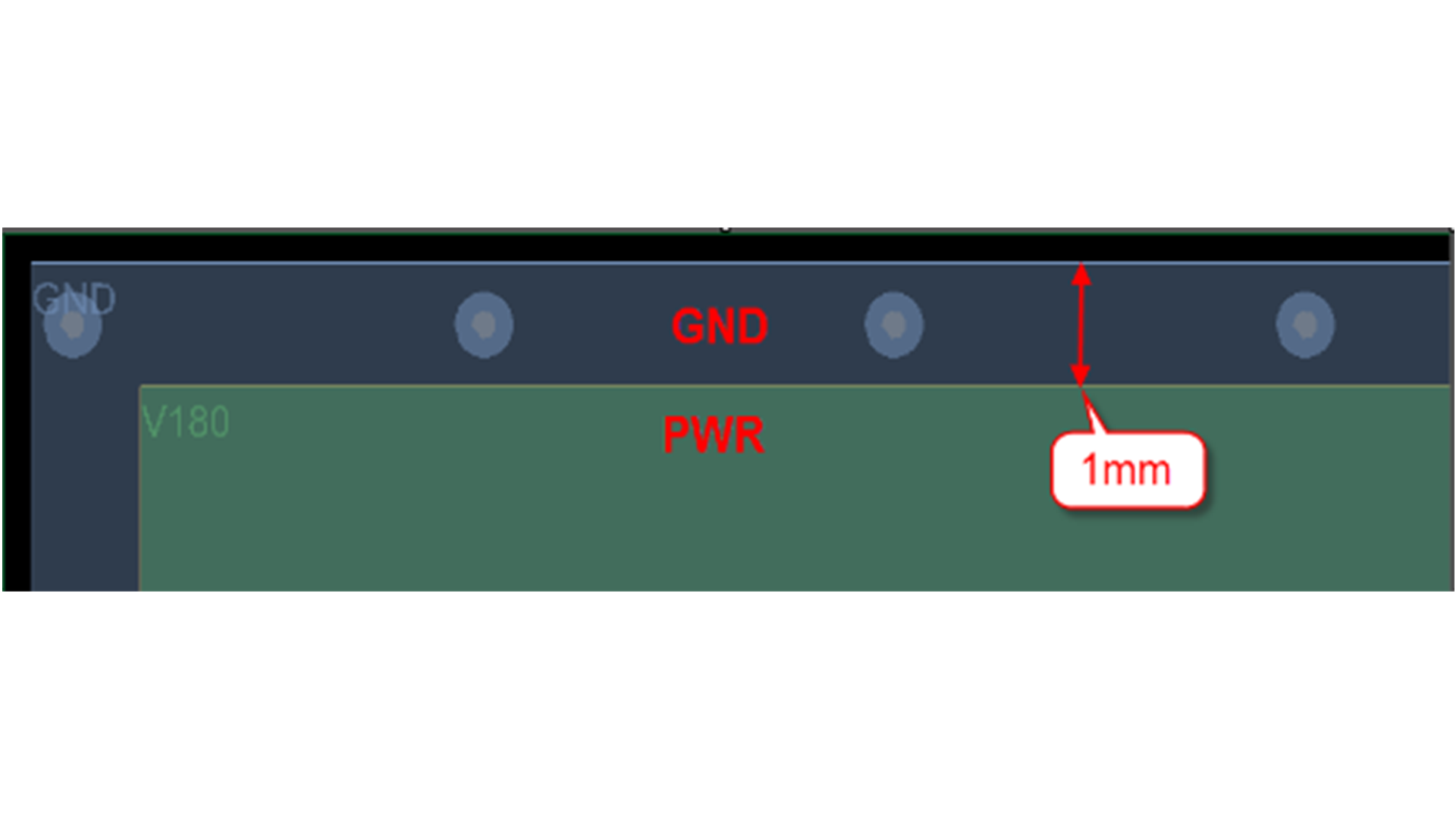
When designing high-speed or high-frequency PCBs, electronics engineers use the 20H principle to meet EMI standards and reduce electromagnetic radiation. This principle requires the power plane to be set back 20H relative to the ground plane, where H represents the distance between the power plane and the ground plane. This also serves to suppress edge radiation. Electromagnetic interference radiates outward at the board's edges. By setting the power plane back, the electric field is conducted only within the confines of the ground plane, effectively improving EMC. A 20H backing can confine 70% of the electric field to the ground edge; a 100H backing can confine 98% of the field. The ground plane should be larger than the power or signal plane to prevent external radiation interference and shield the ground plane from external interference. Generally, setting the power plane back 1mm relative to the ground plane during PCB design is sufficient to meet the 20H principle. To implement the 20H principle, we typically set the power plane back 1mm relative to the ground plane when splitting the plane layers. Shielding ground vias, each 150 mil, are then drilled within the 1mm backing tape, as shown in Figure 1.
Read More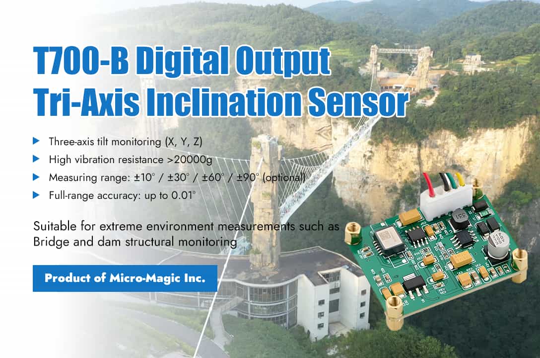
Tilt angle sensors play a crucial role in bridge monitoring, mainly used to measure changes in the tilt angle of bridge structures or their key components relative to the direction of gravity. These minor changes are often important indicators of the health status, load response, foundation settlement, or potential diseases of bridge structures. 1. Main Application Scenarios → Bridge pier/tower tilt monitoring Monitor whether there is slow and uneven settlement of the bridge pier foundation, which may cause the bridge pier to tilt. By using tilt sensors to continuously record angle changes for a long time, trend data can be provided. Real time monitoring of changes in verticality or preset angles during the construction of bridge piers/towers to ensure construction accuracy. → Bearing Displacement and Rotation Monitoring Monitor the rotation angle of bridge bearing under actual load. Abnormal changes in rotation angle may indicate aging, failure, or abnormal constraints of the bearing. By measuring the relative inclination angle between the top and bottom plates of the bearing, combined with the design parameters of the bearing, the sliding displacement of the bearing can be indirectly calculated. → Main Girder Alignment and Deformation Monitoring Although direct deflection measurement typically employs displacement transducers or levels, installing inclinometers at specific locations (e.g., mid-span, pier tops) enables monitoring of rotation changes in girder cross-sections. By integrating these angular measurements with geometric parameters of the girder (such as length), the relative deflection trend at these positions relative to reference points can be calculated. This approach is particularly valuable for long-term structural health monitoring (SHM) and large-span bridges. → Cable Tower/Arch Rib Deformation Monitoring:This process monitors angular changes in cable-stayed bridge towers or arch bridge ribs under load using inclinometers, assessing their global structural stability and deformation status. 2. Advantages of MEMS Tilt Sensors in Bridge Monitoring MEMS tilt sensors are small in size, light in weight, easy to install on structural surfaces or embedded in specific parts, and have minimal impact on the structure itself; MEMS tilt sensors have low cost and lower unit price compared to traditional high-precision tilt meters or fiber optic sensors, making it economically feasible to deploy sensor networks on a large scale and in a dense manner, thereby obtaining more comprehensive structural state information; MEMS tilt sensors have low power consumption and are particularly suitable for wireless sensor networks powered by batteries or energy harvesting, enabling long-term, unmanned monitoring. MEMS tilt sensors are easy to integrate and digitize, typically outputting digital signals directly (such as I2C, SPI, RS485), making it convenient to integrate with data collectors and wireless transmission modules to build automated monitoring systems; MEMS tilt sensors are easy to install and the installation process is relatively simple, usually only requiring a fixed base or magnetic attraction. MEMS tilt sensors have strong dynamic response capabilities, and some high-performance MEMS sensors have sufficient bandwidth to monitor the dynamic response of structures (such as tilt changes caused by vibration) Key Considerations in Applications Bridge monitoring usually requires high accuracy (better than 0.01 ° or even 0.001 ° level) and stability. Although MEMS technology continues to advance, its long-term drift and temperature sensitivity remain challenges, especially when pursuing high-precision applications. It is necessary to carefully select sensor models that meet accuracy requirements and consider temperature compensation and regular calibration strategies. The deformation of bridge structures usually does not change much in angle (often within the range of a few tenths of a degree to a few degrees), but sensors need to have high resolution and high linearity in a small range. At the same time, it is also necessary to consider the larger angles that extreme events (such as strong earthquakes) may produce. Sensors need to be able to withstand drastic temperature changes, humidity, vibration, and possible electromagnetic interference in the bridge environment. Need to choose industrial grade or reinforced packaging products. Tilt angle measurement refers to the angle between the sensor body and the direction of gravity. Therefore, the flatness, stability, and rigid connection with the measured structure of the sensor installation surface are crucial. Any slight deformation or looseness on the installation surface will directly affect the measurement results. Use Case Micro-Magic Inc has produced a series of MEMS tilt sensors to meet the needs of various application scenarios. Including 70 series, T700 series, T7000 series. All series of products are based on industrial design standards, covering both single axis tilt sensors and dual axis tilt sensors. Signal output includes digital and analog (current, voltage) outputs. The measurement accuracy covers the range of medium to high precision. All products support or can be customized with RS232/RS485/RS422/TTL/CAN/MODBUS communication protocols. Micro-Magic Inc has also produced a series of single board tilt sensors, which are convenient for customers to integrate into their own systems. For the special scenario of bridges and dams, Micro-Magic Inc has also launched a series of wireless tilt sensors,. Powered by lithium batteries and based on IoT technology Bluetooth and Zigbee (optional) wireless transmission technology, it avoids application limitations caused by wiring. Conclusion: MEMS tilt sensors, with their unique advantages, provide an economical, efficient, and easy to deploy local angle monitoring method for bridge structural health monitoring. It plays a critical role in monitoring areas such as pier inclination, bearing rotation, and deformation trends of main girders, especially suitable for large-scale deployment and long-term automated monitoring. With the advancement of technology and the improvement of data processing capabilities, its application in bridge monitoring will become more in-depth and intelligent. T700-A T700-B T7000-J
Read More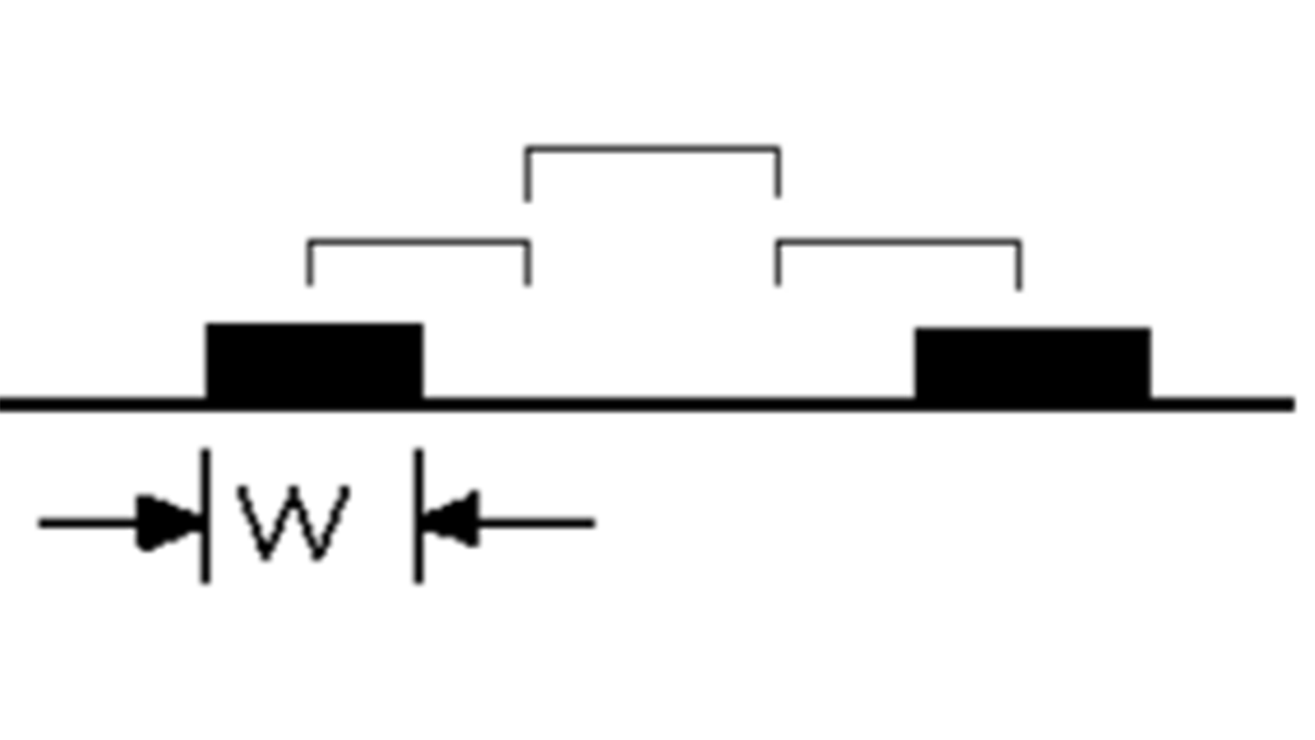
To ensure signal routing quality and prevent crosstalk during PCB design, we maintain a spacing of three times the line width between signal traces. As shown in Figure 1, this spacing refers to the center-to-center spacing of the traces. Because line width is expressed in English as "width," this rule is often referred to as the 3W principle. When the center-to-center spacing of traces is at least three times the line width, 70% of the inter-line electric fields are guaranteed to be free of interference. If 98% of the inter-line electric fields need to be free of interference, the 10W rule can be used. The 3W principle is a PCB layout principle that designers can adhere to without requiring additional design techniques. However, this design approach consumes significant area and can make routing more difficult. The fundamental starting point for the 3W principle is to minimize coupling between traces. This principle can be expressed as follows: the distance between traces (the distance between trace centers) must be three times the width of a single trace. Alternatively, the distance between two traces must be greater than twice the width of a single trace. For example, if a clock line is 6 mil wide, other traces can only be routed 2 x 6 mils away from this trace, or the edge-to-edge spacing must be greater than 12 mils. The 3W principle is easily implemented in PCB design by ensuring that the center-to-center spacing between traces is three times the trace width. For example, if a trace is 6 mil wide, then in Allegro, the line-to-line rule can be set to 12 mils to meet the 3W principle. The spacing in the software is calculated based on the edge-to-edge spacing, as shown in Figure 2.
Read More
The application of MEMS inertial measurement units (IMU) in the industrial field mainly focuses on high-precision motion control, equipment monitoring, and automated production. Choosing a suitable MEMS IMU in the industrial application field requires comprehensive consideration of accuracy, environmental adaptability, interface compatibility, and cost-effectiveness. The application of MEMS IMU in the field of industrial robots and automation mainly focuses on attitude feedback and control, AGV/AMR navigation, and vibration monitoring and diagnosis. In the application of attitude feedback and control, MEMS IMU provides real-time attitude (pitch, roll, yaw) and angular velocity information for robot joints, end effectors or mobile platforms, achieving precise motion control, path planning and collision prevention. In the application of AGV/AMR navigation , MEMS IMU is integrated with wheel speed sensors, LiDAR, and visual sensors to provide dead reckoning functionality. When the external reference is temporarily lost, IMU can maintain short-term positioning and heading, improving the robustness and continuity of navigation. In the application of vibration monitoring and diagnosis, MEMS IMU is installed on robot joints, key structures, or motors to monitor the vibration spectrum and amplitude during operation, for predictive maintenance, and to identify early faults such as bearing wear, imbalance, and misalignment. The requirements for MEMS IMU in the field of industrial robots and automation mainly focus on the following aspects: 1. Requirements for static performance indicators (high precision) Zero bias stability is the most important indicator of static performance, and low zero bias stability means that the long-term accuracy of attitude estimation (pitch, roll, yaw) is crucial. When robots run for long periods of time or AGVs navigate accurately, low zero bias drift is the core to ensure attitude accuracy. The zero bias stability of gyroscopes usually requires <1°/h, and high-end applications require <0.5°/h. The zero bias stability index of accelerometers requires <1 mg. In addition, the angle random walk reflects the white noise characteristics of the gyroscope output, which determines the rate at which the angle integration error increases over time. Low ARW is the foundation for achieving high-precision posture, especially in a short period of time, and is particularly critical for motion control of high-speed and high dynamic robots. Taking the high-performance MEMS IMU U6300 series and U7000 from Micro-Magic Inc as an example: Index item U6300-A U6300-D U7000 Unit Gyro Bias instability 0.5 0.1 0.1 °/h Random walk 0.02 0.05 º/√hr Zero bias stability (10s) 1 3 °/h Accl Bias instability 10 15 μg Random walk 0.02 0.01 m/s/√hr Zero bias stability (10s) 100 100 μg 2. Dynamic performance requirements (high bandwidth, large range) The joint motion frequency of industrial robots is high, and the vibration frequency at the end of the robotic arm may be even higher. High bandwidth is crucial for accurately capturing fast motion and vibration. Usually, the bandwidth needs to be greater than 100 Hz, even hundreds of Hz. In addition, robots can quickly start and stop, collide, or AGVs can travel on uneven roads. Overload can cause data saturation distortion, therefore MEMS IMUs are required to have a sufficiently wide range. Typically, gyroscopes may require ± 300°/s to ± 2000°/s or higher, while accelerometers may require ± 2g to ± 50g or higher. Taking the products U3600, U5000, and U6488 from Micro-Magic Inc as an example: Index item U3600 U5000 U6488 Unit Gyro Range ±2000 ±400 ±450 °/s 3dB Bandwidth 116 250 400 Hz Accl Range ±12 ±10 ±20 g 3dB Bandwidth 145 100 268 Hz 3. Environmental adaptability requirements (excellent resistance to vibration and impact) The industrial environment is full of vibrations (motors, gears, conveyor belts, etc.). IMU must be able to suppress these vibration interferences and avoid outputting erroneous data (especially gyroscopes that are sensitive to linear vibrations and generate G-sensitive errors). Good mechanical design (such as damping) and advanced signal processing algorithms are required. Ensure that the equipment is not damaged and its performance is not permanently degraded when dealing with unexpected collisions, falls, or high impact operations. It usually needs to withstand impacts of thousands of g. Taking the products U3500,U3600 and U3700 from Micro-Magic Inc as an example: Index item U3500 U3600 U3700 Anti-Vibration(g,Rms) 1.0mm(10Hz-58Hz) &≤20g(58Hz-600Hz) Shock(g) 2000, <1ms Environment protection RoHS Directive 2011/65/EU EMC LVD Directive 2014/35/EU Drop test Free fall 3 times on a 75cm high experimental platform Temperature shock Raise the temperature from -40 to 85 ℃ within 1h, 5 times 4. System integration and practicality MEMS IMUs have been increasingly widely used in industrial and military fields due to their small size, light weight, and low power consumption. Miniaturization allows IMUs to be easily embedded into robot joints, linkage ends, compact AGV bodies, and even tool interiors without significant burden or design changes; Lightweight design minimizes the impact of IMU on the load capacity and motion performance of robots, especially for high-speed, high-precision, or collaborative robots; The low power consumption of IMU extends the battery life of mobile robots and wireless sensor nodes, reducing the overall energy consumption and heat dissipation requirements of the system. Taking the products U300, U3500 and U3000 from Micro-Magic Inc as an example: Index item U300-B U3500 U3000 Unit Dimension 22.4*22.4*7.4 22*22*10 59.6*59*23.5 mm Weight 7 8 120 g Power Consumption 0.3 0.3 0.6 W Voltage 3.3 3.3 5 V Conclusion Industrial grade MEMS IMUs need to achieve a high level of balance on these stringent indicators in order to meet the comprehensive requirements of modern industrial robots and automation systems for perception accuracy, reliability, real-time performance, and robustness. U3500 U5000 U6000
Read More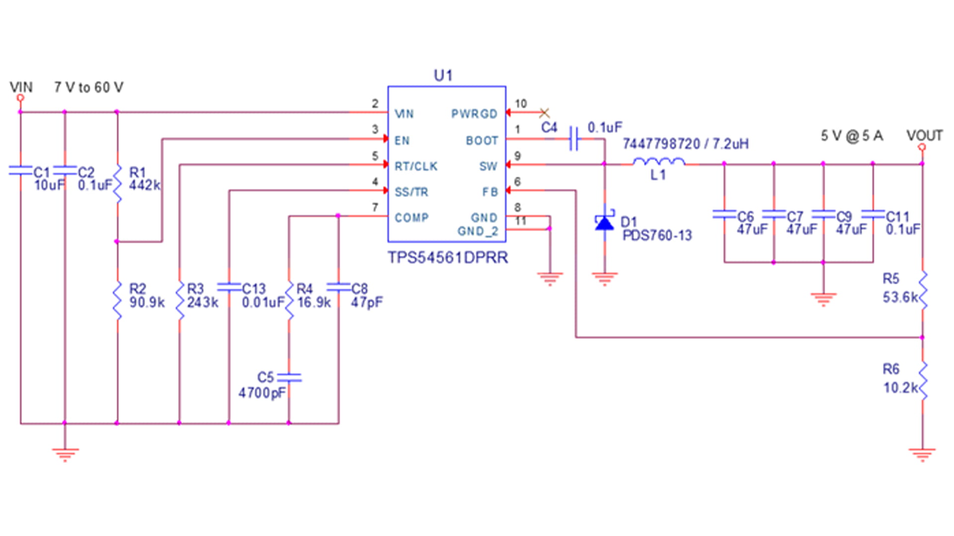
Inrush current is a transient, high current generated when a power supply or device is powered on. In our power supplies and electronic systems, inrush current is undesirable because it can cause device overstress and damage. Buck switching power supply circuits use a soft-start circuit to control the current rise rate during system startup, gradually delivering power to the load and mitigating the impact of inrush current on the system. The soft-start function of a buck power supply is achieved by configuring a soft-start capacitor. This effectively suppresses inrush current, preventing the output capacitor's charging current from exceeding the switching power supply's current limit during startup. This reduces the current surge in the switching circuit itself and downstream loads, and minimizes input voltage drops. Furthermore, a properly configured soft-start time ensures a smooth output voltage rise, avoiding fluctuations . Let's take TI's TPS54561DPRT chip as an example. Its internal functional block diagram is shown in Figure 1. The TPS54561DPRT implements soft-start by connecting an external capacitor to the SS/TR pin. The volt-ampere relationship of a capacitor is expressed as I = C * dV / dt. This shows that the larger the capacitance, the higher the voltage, and the shorter the charging time, the greater the charging current. In other words, for a given capacitance, the magnitude of the capacitor charging current is proportional to the rate of change of the voltage. A typical buck switching power supply device implements configurable soft-start time by connecting an external soft-start capacitor CSS to the soft-start pin SS. The internal pull-up soft-start charging current source ISS charges the soft-start capacitor CSS and then compares it with the reference voltage VREF to determine the end of the soft-start process. According to the capacitor charging formula (I = C*ΔV/ΔT), the time TSS required for the voltage on the soft-start capacitor to charge from zero to VREF is: TSS_SET = CSS * VREF/ISS (Equation 1) For a buck converter circuit, assuming the output voltage setpoint is VOUT, the output capacitor is COUT, and the inrush current charging the output capacitor is IINRUSH, the time required for the voltage on the output capacitor (i.e., the output voltage) to rise from zero to the setpoint VOUT is TSS_OUT. Using the capacitor charging formula, we get: TSS_OUT = COUT * VOUT/IINRUSH (Equation 2) The startup requirement for a switching power supply is that the voltage on the soft-start capacitor must charge from zero to VREF within the soft-start time TSS_SET, and the voltage on the output capacitor must charge from zero to the setpoint VOUT within the same timeframe. Therefore, we get: TSS_SET = TSS_OUT (Equation 3) The final formula for calculating the soft-start capacitor is: (Equation 4) When a switching converter starts up, the current that charges the output capacitor is conventionally referred to as the inrush current, IINRUSH. This current is typically 5% to 10% of the switching converter's maximum load current, IOUT,MAX. If the inrush current, IINRUSH, is 5% of the switching power supply's maximum output current, IOUT,MAX, then IINRUSH = 5% × IOUT. Substituting IINRUSH = 5% × IOUTMAX into Equation 4 yields the following expression for the soft-start capacitor, CSS: (Equation 5) Taking the TPS54561DPRT chip as an example, the actual calculation data is as follows: Requirements: VOUT = 5.0V, COUT = 3 * 47uF = 141uF, IOUT,MAX = 5.0A Parameters: ISS = 1.7uA, VREF = 0.8V, IINRUSH = 5% * 5.0A = 0.25A Calculation results: A standard capacitor close to 10nF is used. This is the reason why C13 = 0.01uF in the figure below. Configuring soft-start capacitors is a key step in suppressing inrush current and ensuring system stability. By properly selecting the capacitor capacity, you can protect components while meeting the startup requirements of different scenarios.
Read More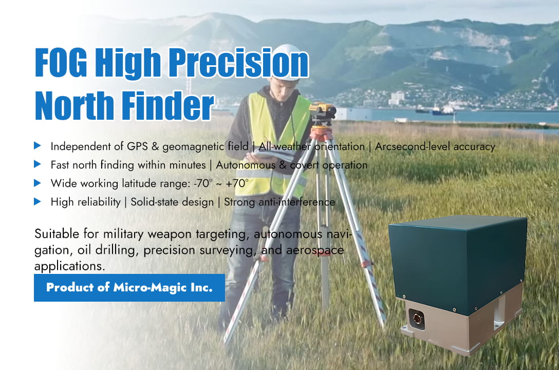
FOG North Finder is a precision instrument that utilizes the Sagnac effect of fiber optic gyroscopes to accurately and autonomously determine the true north direction (geographic North Pole direction). It does not rely on external references such as GPS, astronomical observations, or known reference points, and is not affected by geomagnetic field interference, which is its core advantage. Core Usage (1) Initial alignment and establishment of azimuth reference: This is the most important function. Provide initial orientation reference (true north direction) for various platforms or systems that require knowledge of their absolute direction. (2) Orientation maintenance and autonomous navigation: After knowing the initial position and direction, combined with sensors such as accelerometers, short-term high-precision autonomous inertial navigation can be performed, especially in GPS denied environments. Main Application Scenarios (1) Military field (core applications): ●Weapon system targeting and orientation: FOG North Finder provides fast and covert autonomous north finding for artillery, rocket launchers, and missile launch vehicles, establishing precise shooting reference directions, significantly reducing reaction time, and improving strike accuracy. Provide high-precision azimuth benchmarks for the main guns and fire control systems of tanks and armored vehicles. Provide rapid targeting for shore/ship to ship missile systems. ●Platform orientation and stability: FOG North Finder provides accurate azimuth reference for radar beam pointing of radar systems (ground, vehicle, and ship), ensuring target detection and tracking accuracy. Provide directional reference for the pointing of infrared, laser and other optoelectronic equipment in the electro-optical reconnaissance/aiming system. Provide fast alignment for large directional communication antennas. ● Initial alignment of vehicles/ships: FOG North Finder quickly determines the direction of travel reference for armored vehicles and self-propelled artillery when activated. Provide accurate initial orientation input for inertial navigation systems when submarines, surface vessels depart, float, or require recalibration. (2) Civilian field: ● Petroleum geological exploration: In the measurement while drilling, FOG North Finder is installed near the drill bit to measure the azimuth angle (combined with dip angle) of the borehole in real-time and with high precision. It is a key technology for directional drilling and horizontal drilling, greatly improving drilling efficiency and oil and gas recovery. This is a very important application in the civilian field. ● Geodetic surveying and precision engineering surveying: In areas without GPS signals or signal differences (tunnels, canyons, urban canyons, indoors), FOG North Finder provides high-precision azimuth benchmarks for measuring equipment such as total stations and laser trackers. FOG North Finder provides directional functionality for deformation monitoring systems in large-scale projects such as bridges, dams, and high-rise buildings. FOG North Finder can also establish a measurement control network independent of GPS. ● Aerospace: In the initial alignment and navigation of large drones, FOG North Finder provides the drone with a fast and autonomous takeoff reference direction, and assists in navigation in the event of GPS failure. FOG North Finder provides directional functionality for ground testing and maintenance of aircraft, especially helicopters. FOG North Finder can also assist large satellite antennas in quickly and accurately pointing. Why Does FOG North Finder Have Advantages In These Scenarios? ● Strong autonomy: completely independent of external signals (GPS, geomagnetic), can work at any location and any time. ● Strong anti-interference ability: not affected by electromagnetic interference or metal environments (compared to magnetic compasses), able to work normally in complex electromagnetic environments and near steel structures. ● Fast startup: It can usually complete the search for north within seconds to minutes, much faster than traditional gyroscopic theodolites or astronomical observations. ● High precision: Modern high-precision fiber optic gyroscope north finders can achieve north finding accuracy at the level of arcseconds or even sub arcseconds. ● High reliability and long lifespan: All solid state design, no moving parts (compared to mechanical gyroscopes), shock and vibration resistance, low maintenance requirements. ● Good environmental adaptability: able to work in a wide temperature range and harsh environments (such as high temperature and pressure underground in oil fields). Related Products Suitable For The Above Applications The series of FOG north finder produced by Micro-Magic Inc consists of fiber optic gyroscope, accelerometer, mechanical rotation control device, and embedded computer. It is a high-precision inertial instrument that can autonomously indicate azimuth by providing the angle between the carrier and true north without inputting latitude. This method based on fiber optic gyroscope and precision indexing eliminates dependence on external satellite signals (such as GPS) or known reference points, achieving true autonomous, covert, and all-weather north finding. NF2000 NF3000 NF5000 North finding accuracy (1σ) ≤ 0.5°secψ ≤ 0.02°secψ ≤ 0.05°secψ North search time ≤ 5min ≤ 5 min ≤ 3min Tilt accuracy (pitch/roll, 1 σ) ≤ 0.09 ≤ 0.02° ≤ 0.05° Range of tilt measurement -65 ~ +65 -15° ~ +15° -15° ~ +15° Range of azimuth measurement 0 ~ 360 0° ~ 360° 0° ~ 360° Working latitude range -65 ~ +65 -70° ~ +70° -70°~+70° Conclusion The core value of the fiber optic gyroscope north finder lies in providing a fast, autonomous, high-precision, and anti-interference true north direction reference. This makes it an indispensable key equipment in military weapon orientation, autonomous navigation, oil drilling, precision measurement, and other scenarios that require strict directional benchmarks and often cannot rely on external references or harsh environments. With the continuous advancement and cost reduction of FOG technology, its application in civilian fields is rapidly expanding, especially in the fields of autonomous driving, robotics, and high-end measurement. NF2000 NF3000 NF5000
Read More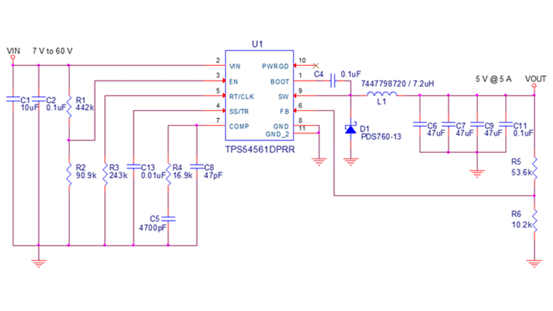
Inrush current is a transient, high current generated when a power supply or device is powered on. In our power supplies and electronic systems, inrush current is undesirable because it can cause device overstress and damage. Buck switching power supply circuits use a soft-start circuit to control the current rise rate during system startup, gradually delivering power to the load and mitigating the impact of inrush current on the system. The soft-start function of a buck power supply is achieved by configuring a soft-start capacitor. This effectively suppresses inrush current, preventing the output capacitor's charging current from exceeding the switching power supply's current limit during startup. This reduces the current surge on the switching circuit itself and downstream loads, and minimizes input voltage drops. Furthermore, a properly configured soft-start time ensures a smooth output voltage rise, avoiding fluctuations. Let's take TI's TPS54561DPRT chip as an example. Its internal functional block diagram is shown in Figure 1. The TPS54561DPRT implements soft-start by connecting an external capacitor to the SS/TR pin. The volt-ampere relationship of a capacitor is expressed as I = C * dV / dt. Therefore, the larger the capacitance, the higher the voltage, and the shorter the charging time, the greater the charging current. In other words, for a given capacitance, the magnitude of the capacitor charging current is proportional to the rate of change of the voltage. A typical buck switching power supply device implements configurable soft-start time by connecting an external soft-start capacitor CSS to the soft-start pin SS. The internal pull-up soft-start charging current source ISS charges the soft-start capacitor CSS and then compares it with the reference voltage VREF to determine the end of the soft-start process. According to the capacitor charging formula I = C * ΔV / ΔT, the time TSS required for the voltage on the soft-start capacitor to charge from zero to VREF is: TSS_SET = CSS * VREF / ISS (Equation 1) For a buck converter circuit, assuming the output voltage setpoint is VOUT, the output capacitor is COUT, and the inrush current charging the output capacitor is IINRUSH, then the time required for the voltage on the output capacitor (i.e., the output voltage) to rise from zero to the setpoint VOUT is TSS_OUT. Using the capacitor charging formula, we get: TSS_OUT = COUT * VOUT / IINRUSH (Equation 2) The startup requirement for a switching power supply is that the voltage on the soft-start capacitor is charged from zero to VREF within the soft-start time TSS_SET, and the voltage on the output capacitor is charged from zero to the setpoint VOUT within the same timeframe. Therefore, we get: TSS_SET = TSS_OUT (Equation 3) The final formula for calculating the soft-start capacitor is: (Equation 4) When a switching converter starts up, the current that charges the output capacitor is conventionally referred to as the inrush current, IINRUSH. This current is typically 5% to 10% of the switching converter's maximum load current, IOUT,MAX. If the inrush current, IINRUSH, is 5% of the switching power supply's maximum output current, IOUT,MAX, then IINRUSH = 5% × IOUT. Substituting IINRUSH = 5% × IOUTMAX into Equation 4 yields the following expression for the soft-start capacitor, CSS: (Equation 5) Taking the TPS54561DPRT chip as an example, the actual calculation data is as follows: Requirements: VOUT = 5.0V, COUT = 3 * 47uF = 141uF, IOUT,MAX = 5.0A Parameters: ISS = 1.7uA, VREF = 0.8V, IINRUSH = 5% * 5.0A = 0.25A Calculation results: A standard capacitor close to 10nF is used. This is the reason why C13 = 0.01uF in the figure below. Configuring soft-start capacitors is a key step in suppressing inrush current and ensuring system stability. By properly selecting the capacitor capacity, you can protect components while meeting the startup requirements of different scenarios.
Read More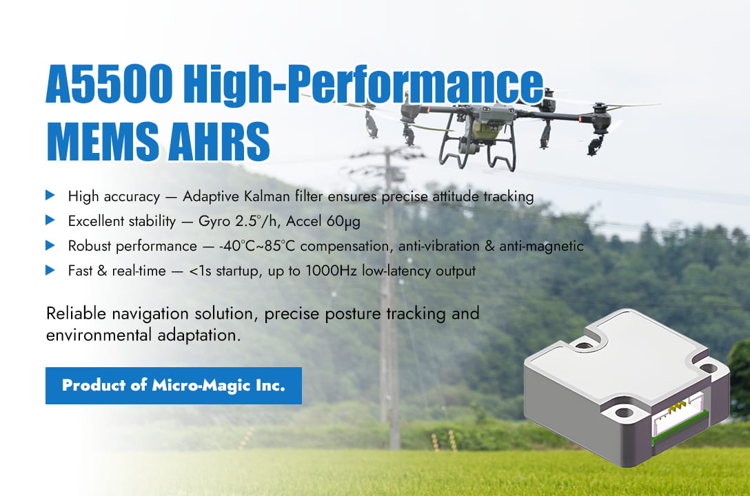
Attitude and heading reference system (AHRS) is a device that utilizes MEMS inertial sensors (accelerometers, gyroscopes) and magnetometers, combined with advanced sensor fusion algorithms (most commonly Kalman filtering and its variants), to calculate real-time attitude information (pitch angle, roll angle, yaw/heading angle) of a carrier (aircraft, vehicle, ship, robot, etc.) relative to the local horizontal plane and in the north direction. The Main Application Scenarios of AHRS 1. Application fields of aviation flight and land vehicles In the attitude stabilization and control system of unmanned aerial vehicles, the flight control system relies on real-time, high-frequency attitude data provided by AHRS to stabilize the aircraft, perform maneuvers (such as turning, climbing, descending), and maintain hovering. This is the most core application of AHRS in unmanned aerial vehicles. Meanwhile, the heading angle provided by AHRS is a key input for unmanned aerial vehicle integrated navigation systems (usually integrated with GPS, barometers, etc.), used for waypoint tracking and autonomous navigation. In the control applications of general aviation aircraft (small aircraft, helicopters), AHRS provides attitude indication and magnetic heading information on the primary flight display (PFD) for pilots. The integration of AHRS with GPS and other systems can provide more reliable and robust navigation solutions for general aviation aircraft. In the stability control of ground vehicles, AHRS is used to detect the roll angle and yaw rate of the vehicle, prevent sideslip and rollover, and provide the auto drive system with vehicle attitude information relative to the road surface for path planning, control decision-making and sensor fusion (such as fusion with camera and radar data). 1. Marine vessels and other advanced technology application fields AHRS monitors the roll and pitch angles of ships for navigation safety, cargo management, or scientific research purposes. In the stability control system of a ship, attitude feedback is provided for stabilizing devices such as anti roll fins and gyro anti roll devices. In ship autopilot/trajectory control, providing heading information is the foundation of ship autopilot. AHRS provides attitude and heading information for ground, aerial, or underwater robots during mobile robot navigation, which is crucial for autonomous movement and positioning. In a robotic arm control system, sensing the posture of the end effector or joint of the robotic arm. In AR/VR systems, the VR headset is equipped with AHRS to track changes in the user's head posture and update the virtual scene perspective. Simultaneously used to capture posture movements of body parts or props (usually requiring higher accuracy and using more professional IMUs). The Main Advantages of AHRS AHRS has the following irreplaceable advantages: → Low cost: The large-scale production of MEMS technology makes AHRS much cheaper than high-precision fiber optic or laser gyro inertial navigation systems (INS), making it widely applicable in consumer and commercial markets such as drones and automotive electronics. → Small size, light weight, low power consumption: MEMS sensors are very compact, and the entire AHRS module can be made very compact and lightweight, with relatively low power consumption, making it very suitable for platforms with limited space, weight, and power consumption (such as small drones and wearable devices). → Quick start and high dynamic response: After starting, it can quickly provide accurate attitude information within seconds to tens of seconds (depending on the convergence speed of the algorithm), without the need for long warm-up periods like mechanical gyroscopes. Capable of quickly responding to the intense maneuvering of the carrier, outputting high-frequency attitude data (usually up to 100Hz or higher), meeting the requirements of real-time control. → Easy to integrate: Typically provides standardized digital interfaces (such as UART, SPI, I2C, CAN, RS232, RS422) for easy integration with other systems (such as flight control computers, navigation computers, displays). Introduction to Related Product Performance The following are the performance indicators of the AHRS series products. Main Parameter A500 A5500 Unit Attitude angles Heading angle 0.2 0.1 ° RMS Pitch/Roll angle 0.2 0.1 ° RMS Attitude ranges Roll ±180 ±180 ° RMS Pitch ±90 ±90 ° RMS Gyroscope Measurement range ±100 ±2000 °/s Angle random walk 0.09 0.6 °/√h Zero bias stability (In-Run) 3 5.1 °/h (Allan) Accelerometer Measurement range ±10/±20/±40 ±12 g Angle random walk 0.03 0.08 (m/s)/√h Zero bias stability (In-Run) 0.03 0.06 mg Magnetometer Measurement range ±8 ±8 Gauss Conclusion AHRS, with its core characteristics of solid-state, low cost, small size, low power consumption, and fast start-up, has become a core attitude sensing device in many fields such as modern drone flight control, small aircraft avionics upgrades, vehicle stability control, ship attitude monitoring and navigation, robot navigation, and VR/AR. Although its absolute accuracy is usually lower than high-end INS systems, its excellent cost-effectiveness and environmental adaptability make it the most widely used attitude reference solution. A500 A5000 A5500
Read More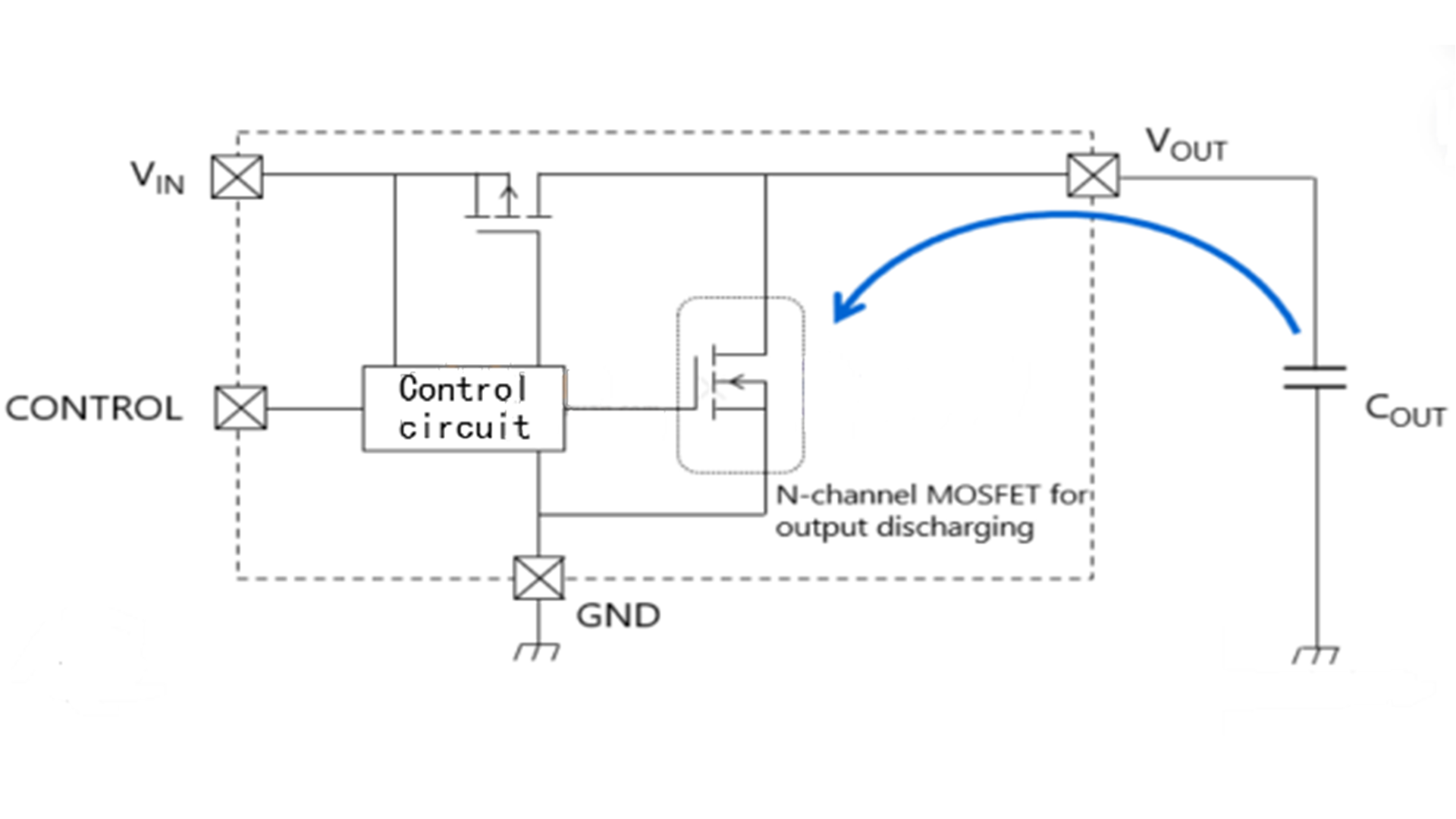
LDOs regulate their output voltage to ensure stable operation under varying load current demands. However, when the load current exceeds the designed range, such as in a short circuit or overload, the excessive current can cause chip overheating or even damage. To address this, overcurrent protection mechanisms have emerged to limit the output current and protect both the LDO and its load. LDOs typically have two overcurrent protection mechanisms: brick-wall current limiting and overcurrent shutdown. 1. Brick-Wall Current Limiting As its name suggests, brick-wall current limiting is a "hard" cutoff mechanism. When the output current exceeds the preset current limit, I_LIMIT, the LDO quickly limits the output current to I_LIMIT. Due to the high load current, the LDO temperature gradually rises. Once the LDO protection temperature is reached, the LDO output is immediately shut down. From the output voltage-output current curve, this resembles a "brick wall" preventing further current increase. For example, the TPS7A16 data sheet indicates that its brick-wall current limit threshold is 105mA (typical). As can be seen from the output voltage-load current curve in the figure above, when the load current exceeds I_LIMIT and triggers the LDO temperature protection, the output voltage drops sharply. This mechanism is typically implemented through an internal current sensing circuit combined with a temperature protection circuit. The LDO's internal structure includes a current mirror to detect current. When the sensed current exceeds the set reference current, the current limit is triggered, the LDO temperature rises, and when it reaches the protection temperature, the power transistor is turned off, cutting off the output. This indicates that brick-wall current limiting is safer during short-term overloads. Its characteristic is that it can tolerate short-term overloads, but if the overload persists, heat accumulation will trigger thermal shutdown. 2. Foldback Current Limit Foldback current limiting is very similar to standard upper-limit limiting. However, its primary purpose is to limit total power dissipation. This means that as VOUT decreases and VIN remains stable, the output current limit is linearly reduced to keep the output transistor within a safe power dissipation limit. Devices such as the TLV717P incorporate and benefit from foldback current limiting because they are primarily housed in ultra-small packages with higher thermal resistance. The output current limit behavior of the TLV717P is shown in Figure 3. As can be seen, since VIN is specified at VOUT + 0.5V, the maximum allowable power dissipation at 25°C is 150mW. After the current limit is exceeded and VOUT begins to decrease (assuming RLOAD is constant), both IOUT and power dissipation decrease. This adds a slight complexity to non-ohmic devices that consume a constant current and can trigger a latched state where the powered device continues to reduce VOUT and the LDO continues to reduce IOUT. 3. Overcurrent shutdown Unlike brick-wall current limiting and foldback current limiting, overcurrent shutdown protection utilizes a fast internal shutdown mechanism. The LDO's internal structure incorporates a current mirror to sense current and a comparator to enable rapid overcurrent output shutdown. When the LDO output current reaches the overcurrent protection current, the LDO directly shuts down. Therefore, current threshold protection is faster than brick-wall current limiting and foldback current limiting. If the LDO output has a large capacitive load, the LDO output will experience a large inrush current, potentially triggering the LDO's overcurrent shutdown, preventing it from starting properly. In this case, an LDO with overcurrent shutdown should not be selected.
Read More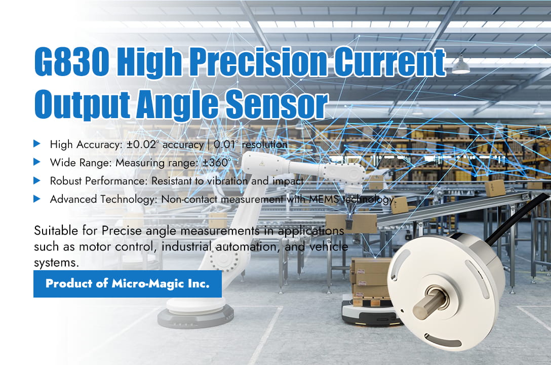
In the field of magnetic sensing technology, three-axis Hall sensors are sparking a precision revolution. This type of sensor achieves true three-dimensional spatial magnetic vector measurement by simultaneously detecting the magnetic field strength in the X, Y, and Z axes, completely breaking through the limitation of traditional single axis Hall sensors that can only detect vertical magnetic fields. The core technology lies in depositing special magnetic flux concentration materials (IMC®) onto the surface of CMOS chips. Enable sensors to capture magnetic field components parallel to the chip surface, combined with high-precision signal chain processing, to achieve 360° full angle position detection. This non-contact measurement method avoids mechanical wear and significantly improves long-term stability and reliability in harsh environments, bringing unprecedented precision control capabilities to modern industry and consumer electronics. Core Technological Advantages: High Precision, Strong Robustness, and Flexibility ■ High Precision and Resolution: The resolution reaches 14 bits (digital signal), equivalent to a resolution of 0.022 °, which is much higher than traditional optical encoders. The typical linearity error is ±1°, and the accuracy is maintained at 10 bits (0.35 °) after temperature drift compensation. The G830 angle sensor even achieves 16 bit ADC accuracy, with an angle error of only 0.02 ° and a temperature drift of 0.002 °/C, reaching the international leading level. ■ Exceptional Environmental Robustness: With strong temperature adaptability, resistance to mechanical tolerances and stray magnetic fields, the working temperature range can reach -40 ° C to+160 ° C, and is insensitive to magnet eccentricity and air gap changes (± 50% tolerance). The third-generation technology can resist stray field interference of 4 kA/m (such as electric vehicle motor magnetic field) and eliminate external interference through differential algorithms. ■ System Integration and Cost Optimization: No PCB packaging, supports direct soldering solutions such as DMP-4 (dual-mode packaging) and SMP-3 (single-mode packaging), eliminates the need for PCB boards, improves EMC/ESD reliability, and reduces system costs. Flexible magnetic circuit design, compatible with various types of magnets with radial/axial magnetization (ferrite, neodymium iron boron, etc.), smaller size and no need for complex calibration. Application Reach: From Automotive Core to Industrial Frontiers In the field of automotive electronics, three-axis Hall sensors have penetrated into key nodes of power transmission: ■ Chassis and safety system: steering wheel torque/steering angle detection (EPS), electronic brake pedal position sensing, accuracy directly affects the stability control efficiency of the vehicle body. ■ Powertrain control: Electronic throttle body, EGR valve angle feedback, with an error of ± 1° to ensure precise emission control. ■ New electric architecture: motor rotor position detection (replacing photoelectric encoders), gearbox gear position sensor. The industrial sector is also experiencing a wave of innovation: ■ Robot joint coding: realizes the detection of robotic arm posture, real-time monitoring of collaborative robot joint angles (0.1° repeatability accuracy), and adapts to industrial environments with anti oil pollution characteristics. ■ Motor control: BLDC motor commutation angle detection, replacing optical encoders. ■ Heavy machinery equipment positioning: Crane arm angle sensing, forklift lifting height detection, agricultural machinery steering angle feedback, IP equivalent protection against dust and water vapor erosion. Three Axis Hall Angle Sensor Related Products Micro-Magic Inc has produced a series of angle sensor products based on three-axis Hall technology, ranging from low to high precision, from low to high cost. Each product undergoes calibration, reverse and anti pulse peak voltage protection, and long-term aging stability testing before leaving the factory. Each process is precise and rigorous, ensuring reliability under different working conditions and long-term use cycles. Angle Sensor Performance Indicators Parameter G803 G810 G830 Unit Measuring range 0~360 ° 0~360 ° 0~360 ° Temperature drift 0.02 0.01 0.002 Resolution 0.05 0.01 0.01 ° Accuracy 1 0.5 0.05 ° Impact resistance 20000g,0.5ms,3 times/axis Anti-vibration 10grms,2~2000Hz Noise 5mV Average working time ≥55000h Output Digital TTL, RS232, RS485, RS422, CAN optional Voltage 0~5V, 0.5-4.5V, 0~10V optional Current 0-20mA, 4-20mA optional Working temperature range -40~85℃ Conclusion The three-axis Hall angle sensor, with its non-contact, high-precision, and multi-dimensional technological advantages, is quietly reshaping the underlying architecture of multiple industries. With the breakthrough of technological bottlenecks, especially the improvement of anti-interference ability and the integration of edge intelligence, this technology will develop towards miniaturization and intelligence, providing a more reliable "spatial perception eye" for the era of Internet of Things.
Read More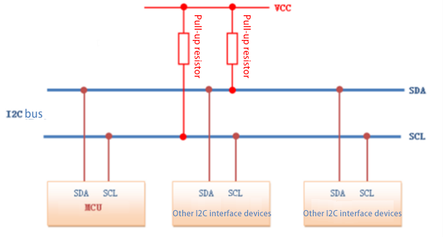
When we design the peripheral circuit of the IIC interface, we usually use the topology diagram with pull-up resistor shown in Figure 1, and its internal structure is the open-drain output shown in Figure 2. The open-drain output level is controlled by an external pull-up and internal logic, allowing the bus to be pulled low and released. The bus open-drain circuit consists of an NMOS transistor, which is turned on and off by a control signal. When the control signal turns on the NMOS transistor, the output is low. When the control signal turns off the NMOS transistor, the output is floating, requiring an external pull-up resistor to output a high level. This structure allows the open-drain gate to flexibly control the bus level while avoiding direct driving of the bus, thus ensuring secure connection and communication between multiple devices. The advantages of using this open-drain output are obvious and are reflected in the following aspects: 1. Short-circuit Prevention If the push-pull configuration is used instead of open-drain, and several devices are connected to the same bus, and an IO on one device outputs a high level while an IO on another device outputs a low level, the VCC and GND connections of these two IOs will short-circuit, causing circuit damage. However, the open-drain configuration eliminates this problem. Regardless of the number of devices connected to the bus, there is no power short-circuit risk. 2. Increase drive capability and reduce power consumption Connecting a pull-up resistor to the drain_output pin allows for level shifting and provides stronger drive capability. This leverages the drive capability of the external circuit to reduce the internal IC drive. When the internal MOSFET of the IC is on, the drive current flows from the external VCC through Rpull-up, the MOSFET, and then to GND. Only a small gate drive current is required within the IC. 3. Use "Wired AND" to determine bus active status Multiple open-drain output pins can be connected to a single line to form an "AND" logic relationship, known as the "wired AND" function. When any one pin goes low, the logic level on the open-drain line becomes 0. This is also the principle used by the I2C bus to determine bus active status. 4. Facilitate output level shifting The transmission level can be changed by varying the pull-up power supply voltage, while the output high level is determined by VDD.
Read Moreleave a message
Scan to Wechat :