Applications

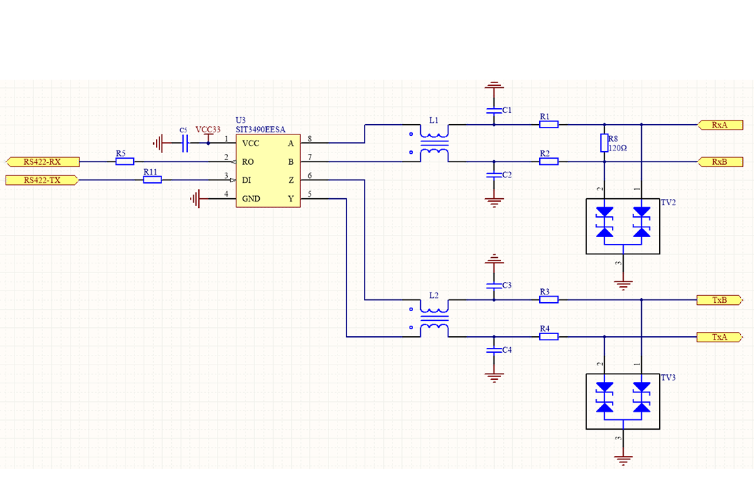
1. RS422 communication principle: (1) RS422 working mode: RS422 supports full-duplex communication mode, that is, data can be transmitted bidirectionally at the same time, that is, two pairs of differential lines are used for sending and receiving respectively, which improves the efficiency and flexibility of communication. (2) Signal level: RS422 uses differential signal to transmit data, that is, two signal lines (one is a positive signal line and the other is a negative signal line) are used to transmit data. It has strong anti-interference ability and can achieve long-distance and high-speed communication. Its differential signal level standard is as follows: ① Transmitter: When transmitting logic "1", the voltage difference between line A and line B is +2V to +6V; when transmitting logic "0", the voltage difference between line A and line B is -2V to -6V. ② Receiving end: It can recognize differential voltages as low as ±200mV. When the voltage of line A is higher than the voltage of line B by more than 200mV, it is recognized as logic "1"; when the voltage of line A is lower than the voltage of line B by more than 200mV, it is recognized as logic "0". (3) Transmission distance: At 115200 baud rate, the maximum transmission distance of RS485 is usually about 1200 meters. Usually the baud rate is inversely proportional to the transmission distance, but the actual distance may vary due to the following factors: ① Transmission line quality: High-quality shielded twisted pair can reduce signal attenuation and interference and extend the transmission distance; ② Electromagnetic environment interference: An environment with strong electromagnetic interference will shorten the transmission distance; ③ Terminal matching resistance: Correctly installing the terminal resistance (usually 120 ohms) can reduce signal reflection, ensure signal integrity, and improve communication quality. If a longer distance is required, consider reducing the baud rate or using a repeater. (4) Load capacity of the transmitter: One RS422 driver can drive up to 10 receivers. (5) Connection method of terminal matching resistor: RS422 can be connected without terminal matching resistor when the distance is short (generally not more than 300 meters). When communicating over long distances, a 120 ohm resistor can be connected at the end of the signal receiving end as the terminal resistor. The terminal resistor can absorb the reflected waves on the network and effectively enhance the signal strength.   (6) Protection of RS422 circuit and suppression of interference: Generally, anti-static (ESD) protection, current limiting protection and suppression of common mode noise are required. The electrical principle is shown in the figure below:   Anti-static (ESD) protection: Connect TVS diodes to the ground on the A and B differential lines respectively to prevent static crosstalk to the subsequent circuit and damage to components. Current limiting protection: Connect a small resistance resistor in series on the A and B differential lines to prevent the signal line from short-circuiting or overcurrent from damaging the interface chip. Suppression of common mode noise: Connect common mode chokes L1 and L2 in series on the A and B differential lines to suppress common mode interference on the line and improve the anti-interference ability of the system. The common mode inductor impedance selection range is 120Ω/100MHz~2200Ω/100MHz, and the typical value is 1000Ω/100MHz. The sending and receiving A and B differential lines are connected to the ground and connected to capacitors to provide a low-impedance return path for interference to suppress common-mode high-frequency noise. The capacitance value selection range is 22PF~1000pF, and the typical value is 100pF. 2. Precautions for on-site use: (1) RS422 signal lines cannot be routed together with strong power lines, and the principle of separation of strong and weak electricity must be followed. (2) The correct connection method of signal lines and ground lines, the A and B lines of the sending end are connected to the A and B lines of the receiving end, and the ground line must also be connected. The signal ground can be an additional unshielded twisted pair or the shielding layer of a shielded twisted pair. The RS422 bus must be reliably grounded at a single point, that is, there can only be one point grounded on the entire RS422 bus, not multiple points, because the reason for grounding is to keep the voltage on the ground wire (usually the shielded wire is used as the ground wire) consistent to prevent common mode interference. If multiple points are grounded, it will be counterproductive. (3) Signal interference causes unstable communication and solutions: If there is sometimes no communication connection on site, this may be that the signal is interfered with, thus affecting the continuity of the signal. This requires the use of shielded twisted pair cables for long-distance transmission, and a 120-ohm impedance matching resistor is connected in parallel at the receiving terminal. (4) Selection of shielded cable: Choose to use ordinary Category 5e shielded twisted pair cables, i.e. network cables.   3. Common problems and solutions of RS422 communication:   Problem Possible cause Solution Communication failure Wrong line connection Ensure A+ and B- are correctly connected   Data loss Transmission distance is too long or rate is too high Reduce baud rate or use relay amplifier Severe interference Electromagnetic interference Use shielded twisted pair and ensure good grounding   Signal reflection No terminal matching Add 120Ω terminal resistor at the end of the bus Multi-device communication abnormality Exceeding the maximum number of receiving devices Reduce the number of receiving terminals or use RS-485 instead

Wheel speed sensors (wheel speed sensors) are often used as auxiliary sensors in inertial navigation systems (INS) to improve navigation accuracy and suppress accumulated errors of inertial sensors. The wheel speed gauge calculates the longitudinal speed of the vehicle by measuring the wheel speed (combined with tire radius and slip ratio correction), providing independent speed information. When GPS signals are lost (such as in tunnels or underground garages), INS can continuously estimate the vehicle's position through dead reckoning by combining the speed data of the wheel speed meter, and compare it with the accelerometer integration results of INS to correct the speed error. In heading calculation, the wheel speed gauge can indirectly calculate the rate of change of heading angle by measuring the speed difference between the left and right wheels (wheel speed difference), providing compensation for the calibration of inertial navigation heading angle. Taking the change of heading angle as an example, this article briefly introduces how to indirectly calculate the rate of change of heading angle through the data obtained from the wheel speed meter.   1.  Basic principles   Assuming that the vehicle has a rigid body and only moves in a horizontal plane (ignoring pitch and roll), there is no lateral slip at the contact point between the tires and the ground (only considering longitudinal rolling), and the left and right wheelbase (wheel spacing) is a fixed value. The relationship between wheel speed and linear speed is shown in the following equation:       When the vehicle turns, the left and right wheels move around the same instantaneous center of rotation (ICR), The vehicle angular velocity   is the rate of change in heading angle. The difference in linear velocity between the left and right wheels is generated by the rotation of the vehicle around the ICR, satisfying the following relationship:   where：  : the wheel spacing ，  : the turning radius Therefore, there is a difference in linear velocity between the left and right wheels：    The rate of change in heading angle (angular velocity) is:                           2.  Factors affecting the measurement accuracy of wheel speed gauge and algorithm correction   In practical applications, the following issues may lead to inaccurate measurement data of the wheel speed gauge, affecting the error compensation of the azimuth angle in INS. a)   Track B The actual wheelbase may vary due to load or suspension deformation and requires regular calibration. The above formula assumes that the left and right wheels are symmetrical, so the model needs to be adjusted for asymmetric vehicles. b)   Slip and error compensation In wet and slippery road surfaces or off-road environments, or when the vehicle accelerates or brakes rapidly, it may cause tire slippage, resulting in a wheel speed difference that does not match the true angular velocity. Therefore, it is necessary to combine the acceleration and angular velocity data of IMU (Inertial Measurement Unit) to detect the slip state; Dynamically adjust the weight of the wheel speed gauge through multi-sensor fusion algorithm (Kalman filter algorithm) to reduce the impact of slip-on navigation.   3.   Actual use cases   I3500 is an integrated navigation system (GNSS/INS) produced by Micro-Magic Inc, consisting of high-performance MEMS sensors, high-precision GNSS systems, and high-performance microprocessors. Can be connected to an external odometer, DVL and other auxiliary navigation information, with built-in high reliability integrated navigation algorithms, can output real-time information such as speed, position, and attitude of the carrier.     Data input/output Parameters Describe Data Output NMEA/RTCM/Novtel SPAN Binary Protocol Data Content Euler angle, velocity, position, acceleration, angular velocity Fusion Algorithm Extended Kalman Filter External Sensor Mileage meter, GNSS, DTU Integrated navigation accuracy index Position Position Accuracy Velocity Accuracy Pitch/Roll Accuracy   Mileage Meter Access 1cm 0.03m/s 0.1° 1m 0.1m/s 0.1° 6m 0.1m/s 0.2°   Conclusion   The wheel speed gauge complements the inertial navigation system by providing independent speed information, significantly improving the navigation reliability of vehicles in complex environments. Its core values are reflected in: a. Short term accuracy: high-frequency speed data suppresses INS error accumulation. b. Redundant design: Maintain basic navigation capability in the event of GPS failure. c. Cost effectiveness: Significant improvement in navigation performance achieved at a lower cost. In the future, with the advancement of multi-sensor fusion algorithms such as deep learning assisted filtering, The application of wheel speed sensors in autonomous driving and unmanned systems will be further deepened. I3500 High Accuracy 3-Axis MEMS Gyro I3500 Inertial navigation system   I3700 High Accuracy Agricultural Gps Tracker Module Consumption Inertial Navigation System Mtk Rtk Gnss Rtk Antenna Rtk Algorithm  

"An in-depth analysis of the testing methods for the bias (zero bias) and scale factor of quartz flexible accelerometers is provided, including specialized techniques such as four-point rolling test and two-point test, as well as the calculation formula for temperature sensitivity. This is applicable to high-precision applications such as inertial navigation and spacecraft." The bias (zero bias) and scale factor of quartz flexible accelerometers directly determine the measurement accuracy and long-term stability of the accelerometer, especially in high-precision application scenarios such as inertial navigation and attitude control. Therefore, they are two key performance indicators for evaluating quartz accelerometers.   The core significance of bias (zero bias) lies in its inherent system error of the accelerometer, which directly leads to the fundamental deviation of all measurement results. For example, if the zero bias is 1 mg, the measured value will add this error regardless of the actual acceleration. Zero bias will also drift with factors such as time, temperature, and vibration (zero bias stability). In inertial navigation systems, zero drift is continuously amplified through integration operations, resulting in cumulative errors in position and velocity. The temperature characteristics of quartz materials can also cause zero bias to change with temperature (zero bias temperature coefficient), so temperature compensation algorithms are needed to suppress this effect in high-precision applications. Scale factor refers to the proportional relationship between the output signal of an accelerometer and the actual input acceleration. The error in scale factor can directly lead to proportional distortion of the measurement results. The stability of scale factor directly affects system performance in high dynamic range or variable temperature environments. In the acceleration integration operation of inertial navigation, the scale factor error will be integrated twice, further amplifying the position error.   Therefore, the reason why bias and scale factor have become key performance indicators of quartz flexible accelerometers is that they are both fundamental error sources and key constraints on long-term stability. In system level applications, the performance of these two directly determines whether the accelerometer can meet the requirements of high precision and high reliability, especially in scenarios such as unmanned driving, spacecraft, submarine navigation, etc. where there is zero tolerance for errors   The bias test can be conducted through two methods: four point rolling test (0°，90°，180°，270°positions) or two-point test (90°，270°positions). The scale factor test can be conducted through three methods: four point rolling test (0°，90°，180°，270°positions), two-point test (90°，270°positions), and vibration test. Taking the four-point rolling test method as an example, this article explains how to obtain the bias and scale factor of an acceleration sensor.     1. Testing methods for bias and scaling factors:   a) Install the accelerometer on a specific test bench (multi tooth indexing head). b) Start the test bench c) Rotate the test bench clockwise to the 0°position, stabilize it, and record the output of multiple sets of tested products according to the specified sampling frequency. Take the arithmetic mean as the measurement result; d) Rotate the test bench clockwise to the 90°position, stabilize it, and record the output of multiple sets of tested products according to the specified sampling frequency. Take the arithmetic mean as the measurement result; e) Rotate the test bench clockwise to the 180°position, stabilize it, and record the output of multiple sets of tested products according to the specified sampling frequency. Take the arithmetic mean as the measurement result; f) Rotate the test bench clockwise to the 270°position, stabilize it, and record the output of multiple sets of tested products according to the specified sampling frequency. Take the arithmetic mean as the measurement result; g) Rotate the test bench clockwise to the 360°position, then counterclockwise to make the rotation angles at 270°, 180°, 90°, and 0°positions. After stabilization, record the output of multiple sets of tested products according to the specified sampling frequency, and take the arithmetic mean as the measurement result. h) Calculate the bias and scaling factor of the tested product using the following formula (1) and (2). K0 =    -------------------------------------- (1)   K1 =   -------------------------------------- (2)        Where:         K0 -------Bias         K1 -------Scale factor         -------The total average of forward and reverse readings at 0°position         -----The total average reading of forward and reverse rotation at 90°position         --- The total average reading of forward and reverse rotation at180° position         --- The total average of readings for forward and reverse rotation at 270°position   2. Test method for bias temperature sensitivity and scale factor temperature sensitivity a) Start the test bench b) Calculate the bias and scaling factors at each temperature point using the formulas (1) and formulas (2) at room temperature, the upper limit operating temperature specified by the accelerometer, and the lower limit temperature specified by the accelerometer. c) Calculate the temperature sensitivity of the accelerometer using the following formula (3) and (4):      ---------------------(3) where： ---- Bias temperature sensitivity ----Bias of upper limit temperature of sensor ----Bias of sensor room temperature -----Bias of the lower limit temperature of the sensor ------Upper limit temperature ------Room temperature -------Lower limit temperature        ---------------------(4) Where: ----Scale factor temperature sensitivity ------Scale factor ----Scale factor for the upper limit temperature of the sensor ----Scale factor of sensor room temperature -----Scale factor for the lower limit temperature of the sensor ------Upper limit temperature ------Room temperature -------Lower limit temperature AC-1 Quartz Flexible Accelerometer   AC-4 Quartz Flexible Accelerometer  

Fiber optic gyroscope is based on Sagna effect and is widely used for measuring angular velocity in navigation and attitude control. Key indicators typically include zero bias stability, scaling factor, random walk, bandwidth, noise, temperature characteristics, and so on. By measuring these indicators, the performance of fiber optic gyroscopes can be comprehensively evaluated, and system design and compensation algorithms can be optimized based on these data.   1. Zero Bias Series Testing 1.1 Bias Definition： The average equivalent angular velocity output of a fiber optic gyroscope when there is no angular velocity input. Test Equipment: horizontal reference device, fiber optic gyroscope output measurement recording device. Test method: Fix the fiber optic gyroscope on a horizontal reference, with the input axis (IRA) pointing in the east-west direction. Record output data for at least 1 hour after power on, with a sampling frequency that meets the Nyquist criterion (≥ 2 times the highest frequency of the signal). Calculation formula:                 Where K is the scaling factor, is the average output value.   1.2 Bias Stability Definition: The degree of dispersion of zero bias output around the mean reflects short-term stability. Test method: Same as bias test, but requires long-term data recording (at least 1 hour). Calculation formula:                   where:  ： Zero bias stability, measured in degrees per hour (° ⁄ h) :  The single-sided amplitude output of the fiber optic gyroscope  at time .   1.3 Bias Repeatability Definition: Perform multiple power tests to ensure consistency of zero bias. Test method: Repeat the zero-bias test for more than 6 times, with power off and cooling to room temperature at intervals between each test. Calculation formula: For each test data, process it according to formula (1), calculate the zero bias, and then calculate the zero-bias repeatability of Q tests according to the following formula.                        Where,   :  Zero bias of the i-th test; :  Zero bias   1.4 Bias Temperature Sensitivity Definition: Zero bias drift caused by temperature changes. Test method: Set different temperature points (covering the working temperature range) inside the temperature control box, and maintain a constant temperature for 30 minutes at each temperature point. Measure the zero bias at each temperature point and calculate the deviation from the room temperature zero bias. Calculation formula: The test data is processed according to formula (1), and the zero bias of the fiber optic gyroscope at room temperature and each test temperature point is calculated separately. The zero bias temperature sensitivity of the fiber optic gyroscope is calculated according to the following formula:                             ：The i-th test temperature.  ：room temperature   2. Scale Factor Series Testing 2.1  Scale Factor Definition: Linear proportional relationship between output signal and input angular velocity Test equipment: high-precision rate turntable (error<1/3 of the tested gyroscope index) Test method: Select ≥ 11 angular velocity points (including the maximum input angular velocity) uniformly in both forward and reverse directions. Record the mean output of each point and fit a straight line using the least squares method. Calculation formula: Let be the average output of the fiber optic gyroscope at the jth input angular velocity, and the scaling factor calculation method is as follows:                                               The linear model for establishing the input-output relationship of fiber optic gyroscope is as follows:                     Using the least squares method to calculate K,                               Where ∅ is the rotational speed of the speed turntable, measured in degrees per second (° ⁄ s)   2.2 Scale factor nonlinearity Definition: Output the maximum deviation relative to the fitted line. Calculation formula: According to the above method, the input-output relationship of the fiber optic gyroscope is represented by fitting a straight line as follows:               Calculate the point-by-point nonlinear deviation of the output characteristics of the fiber optic gyroscope according to the following formula:                   Calculate the scaling factor linearity according to the following formula, and create the nonlinear deviation curve of the fiber optic gyroscope output (the horizontal axis represents the input angular velocity, and the vertical axis represents the nonlinear deviation)                   2.3 Scale factor temperature sensitivity Test method: Test the scaling factor at different temperature points and calculate the deviation caused by temperature changes. Calculation formula: The test data is processed according to the calculation method of scale factor, and the scale factor of the fiber optic gyroscope at room temperature and each test temperature point is calculated separately. The temperature sensitivity of the scale factor is calculated according to the following formula:                 3. Random Walk Coefficient (RWC) Definition: Integral angular velocity error caused by white noise output. Test method: Short time (tens of seconds) high-frequency sampling, analyze Allan variance. Formula for calculating Allan variance: a) There are n initial sample data of fiber optic gyroscope output values obtained at the initial sampling interval time . According to the calculation formula for gyroscope zero bias, the output angular velocity of each fiber optic gyroscope output value is calculated to obtain the initial sample data of output angular velocity, as shown in the following formula:               b) For continuous data of n initial samples, k continuous data are grouped together, and the time length of the array is set to , where τ equals , 2 ,  Calculate the average value of the array data for each time length. c) Find the average difference between two adjacent arrays:           d) Calculate the variance of a set of random variables:   …… (17) Repeat the above process with different values of, and obtain a curve in the double logarithmic coordinate system, which is called the Allan variance curve. Using the Allan variance model below, the coefficients are obtained through least squares fitting, and then the random walk coefficient RWC is calculated:                   Conclusion: The key indicator testing of fiber optic gyroscope is a bridge connecting research and development with practical applications. By quantitatively verifying performance, ensuring reliability, and meeting standard compliance, it ensures its "precision, stability, and usability" in military and civilian high-precision fields, while laying the foundation for technological innovation and cost optimization. GF2X64 Dual-Axis Low Precision Fiber Optic Gyroscope GF-60 Medium and Low Precision  Fiber Optic Gyroscope GF3G90 Tri-Axis Fiber Optic Gyroscope    

Electronic compass is an important navigation tool that can provide real-time heading and attitude of moving objects. Calibration of an electronic compass is a crucial step in ensuring the accuracy of its directional measurement.   1. Calibration principle of electronic compass The electronic compass determines direction by measuring the components of the geomagnetic field. The calibration process is actually "magnetic field ellipse fitting": a) Collect magnetic field data  in all directions when the device rotates. b) Generate compensation parameters by calculating hard iron interference (fixed offset) and soft iron interference (scaling and cross coupling) through algorithms. c) Automatically apply compensation during subsequent measurements to fit the magnetic field data into a sphere centered at the origin, improving directional accuracy.   2. Calibration method for electronic compass The calibration methods for electronic compasses mainly include two methods: planar calibration and three-dimensional 8-shaped calibration. (1) Plane calibration method For the calibration of the XY axis, the device equipped with a magnetic sensor will rotate on its own in the XY plane, which is equivalent to rotating the Earth's magnetic field vector around the normal passing point O(γx,γy) perpendicular to the XY plane. It represents the trajectory of the magnetic field vector projected in the XY plane during the rotation process. This can find the position of the center of the circle as (Xmax+Xmin)/2, (Ymax+Ymin)/2. Similarly, rotating the device in the XZ plane can obtain the trajectory circle of the Earth's magnetic field on the XZ plane, which can calculate the magnetic field interference vector γ (γx, γy, γz) in three-dimensional space. After calibration, the electronic compass can be used normally on the horizontal plane. However, due to the angle between the compass and the horizontal plane, this angle can affect the accuracy of the heading angle and requires tilt compensation through acceleration sensors. (2) Stereoscopic 8-shaped calibration method Usually, when a device with sensors rotates in various directions in the air, the spatial geometric structure composed of measured values is actually a sphere, and all sampling points fall on the surface of this sphere, as shown in the following figure.‌                a) Aerial rotation:  Use calibrated equipment to perform an 8-shaped movement in the air, aiming for the normal direction of the equipment to point towards all 8 quadrants of space. By obtaining sufficient sample points, the center O(γx,γy,γz) is determined, which is the size and direction of the fixed magnetic field interference vector. b) Sample point collection:  When rotating the device in various directions in the air, the spatial geometric structure composed of measurement values is actually a sphere, and all sampling points fall on the surface of this sphere. By using these sample points, the center of the circle can be determined to determine the hard magnetic interference value and perform calibration.   3. Calibration steps for electronic compass (1) Preparation of testing environment Ø Stay away from interference sources: Ensure that there are no large metal objects (such as iron cabinets, vehicles), motors, speakers, or other electromagnetic equipment within 3 meters of the calibration environment. Ø Horizontal placement: Use a level or built-in sensor to adjust to a horizontal state, ensuring that the measurement is based on the horizontal component of the geomagnetic field. Ø Fixed method: Avoid wearing metal watches or rings when holding the device; If it is an embedded device (such as a drone), ensure a stable installation. (2) Enter calibration mode a) Manual triggering: Refer to the product manual, common methods include: n Key combination (such as long pressing the power and function keys for 5 seconds). n Software instructions (select 'Calibrate Compass' through the accompanying app). b) Auto prompt: Some devices automatically prompt calibration when detecting magnetic field anomalies (such as continuously displaying "low precision").   (3) Perform calibration operation a) Horizontal rotation (2D calibration): n Slowly rotate the equipment around the vertical axis (Z-axis) and keep it horizontal. n Ensure uniform rotation speed (about 10 seconds/turn), complete at least 2 turns to cover all directions. b) Three-dimensional rotation (3D calibration, suitable for high-precision equipment): n Rotate around the X (roll), Y (pitch), and Z (yaw) axes in sequence, with each axis rotating at least 360 °. n Example action: After horizontal rotation, flip the device upright and then tilt it back and forth. (4) Verify the calibration results a) Direction comparison method: Point the device towards a known geographic direction (such as using a compass to determine true north) and check if the readings match. b) Software validation: Use map apps or professional tools (such as magnetic field analysis software) to observe directional stability and accuracy. c) Repeat calibration: If the deviation exceeds the nominal error of the equipment (such as ±3°), recalibration and environmental interference inspection are required.   C9-B High Precision CAN Protocol Output 2D Electronic Compass C9-A 40° Tilt Angle Compensation CAN Protocol Output 3D Electronic Compass C9-C High Precision Digital Output 2D Electronic Compass Single Board  

Inertial measurement unit (IMU) is an integrated sensor kit that combines multiple accelerometers and gyroscopes to perform three-dimensional measurements of specific force and angular velocity relative to an inertial reference frame. However, in recent years, IMU has become a general term used to describe various inertial systems, including attitude heading reference systems (AHRS) and INS. IMU itself does not provide any type of navigation solution (position, velocity, attitude) . Normally, inertial sensors can be divided into the following three performance categories:   Marine-grade and Navigation-grade inertial navigation systems :     Marine-grade inertial navigation systems are the highest level of commercial sensors used on ships, submarines, and occasionally on spacecraft. This system can provide a non assisted navigation solution with drift less than 1.8 km/day. The cost of these sensors is as high as $1 million. The performance of navigation grade inertial navigation systems is slightly lower than that of Marine-grade inertial navigation systems, and is usually used for commercial and military aircraft. Its drift is less than 1.5km/h, and its price is as high as $100000. Tactical and industrial inertial sensors: Tactical and industrial grade sensors are the most diverse among these three types of sensors, capable of addressing various performance and cost situations, and their market opportunities are enormous. This category is used for many applications that require high-performance data to be obtained at a lower cost for mass production, commonly found in automatic lawnmowers, delivery robots, drones, agricultural robots, mobile industrial robots, and autonomous ships. Consumer grade sensors: In the commercial market, these sensors are usually sold in the form of separate accelerometers or gyroscopes. Many companies have started combining multiple accelerometers and gyroscopes from different manufacturers to create independent IMU units   Choosing the appropriate inertial sensor (such as accelerometer, gyroscope, magnetometer, or combined IMU/AHRS) requires comprehensive consideration of multiple factors including application scenarios, performance parameters, environmental conditions, and costs.   1. Clarify application requirements   Dynamic range: Determine the maximum acceleration or angular velocity that the sensor needs to measure (for example, a high range gyroscope is required for high-speed maneuvering of a drone). Accuracy requirements: High precision navigation (such as autonomous driving) requires sensors with low noise and low bias. Update frequency: High frequency vibration monitoring requires a sampling rate of>1kHz, while conventional motion tracking may only require 100Hz. Power consumption limit: Wearable devices require low power consumption (such as MEMS accelerometers with ± 10mg noise), while industrial devices can be relaxed. Integration method: Do you need IMU (6-axis) or AHRS (with attitude calculation).   2. Key performance parameters   Accelerometer: Range: ±2g (inclination measurement) to ±200g (impact detection). Noise density:  < 100μg/√ Hz (high precision) vs >500 μg/√Hz (low cost). Bandwidth: It needs to cover the highest frequency of the signal (e.g. mechanical vibration may require >500Hz).   Gyroscope: Zero bias stability: < 1°/h (fiber optic gyroscope) vs 10°/h (industrial MEMS) vs 1000 °/h (consumer grade). Angle random walk (ARW): <0.1°/√h (tactical level) vs 5°/√h (consumer level). Range: ±300°/s (conventional) to ±2000 °/s (high-speed rotation).   Magnetometer: Sensitivity: 0.1μT/LSB (high-precision navigation) vs 0.5μT/LSB (universal). Orthogonal error:  <1° (reduces the influence of soft iron interference).   3. Environmental adaptability   Temperature range: Industrial grade (-40°C~85°C) vs Consumer grade (0° C~70°C). Anti vibration/impact:  For example, automotive electronics need to pass a 5g RMS vibration test. Sealing:  IP67/IP68 protection level (outdoor or humid environment).   4. Interface and power consumption   Digital interfaces: SPI/I2C (embedded systems), CAN (automotive), UART (simple communication). Power supply voltage: 3.3V (low power consumption) vs 5V (industry standard). Power consumption: < 1mA (battery device) vs unlimited (wired power supply).   Micro-Magic Inc is a high-tech company specializing in the production, manufacturing, and research and development of automotive grade and industrial grade inertial sensors. The company's inertial sensor include various series of products such as accelerometers, gyroscopes, magnetometers, inclinometers, IMUs, VRUs, AHRS, and INS+GNSS integrated navigation. Over the years, The company's products have been widely used in various application fields, including automotive, aerospace, marine vessels, industrial automation, and medical equipment. The company's products have the characteristics of high precision, low power consumption, small size, and high reliability, and are widely used in fields such as attitude control, navigation systems, motion tracking, and vibration analysis. At the same time, Micro-Magic Inc are also committed to providing customized solutions for customers to meet the specific needs of different industries U6488 MEMS High Precision Digital Output IMU Sensor U7000 High Precision MEMS IMU U300-A Digital Output High Performance MEMS IMU Sensor  

Fiber optic gyroscopes (FOGs) are highly accurate sensors used to measure angular velocity. They are widely used in fields such as aviation, navigation, and seismic research due to their high precision, sensitivity, and excellent stability. Its core accuracy indicators, including zero bias drift, random walk, and angle measurement error, are the key to evaluating its performance. Detailed explanation of core accuracy indicators Fiber optic gyroscope uses optical fibers as sensing elements to achieve accurate measurement of rotational angular velocity. Its accuracy performance can be comprehensively evaluated through the following three indicators:   (1)    Bias Stability (Drift Rate)   This indicator reflects the output accuracy of the gyroscope in a non rotating state, usually measured by a benchmark accuracy. The zero bias drift of fiber optic gyroscope is extremely low, generally not exceeding 0.2 °/h, ensuring high measurement accuracy.   (2)    Random Walk (Angular Random Walk, ARW)   This indicator measures the stability of the gyroscope output value over a period of time. typically measured in degrees per square root hour (°/√h). For example, the FOG has an ARW of 0.001°/√h. This means that the noise in the gyroscope's output accumulates at a rate of 0.001 degrees per square root of the operating time. (3)     Scale Factor Accuracy   The scale factor accuracy indicates how well the gyroscope's output corresponds to the actual angular velocity. It is usually expressed as a percentage error. For example, The FOG has a scale factor accuracy of 10 ppm (parts per million)**. This means that for every degree per second (°/s) of actual rotation, the gyroscope's output may deviate by up to 0.001%.   Analysis of Factors Affecting Accuracy The accuracy of fiber optic gyroscopes is influenced by various external factors: (1)    Temperature: The sensitive components of fiber optic gyroscopes are sensitive to changes in ambient temperature, which may lead to zero bias drift or increased angle measurement errors. (2)    Vibration: Environmental vibrations can have adverse effects on the accuracy of fiber optic gyroscopes, potentially leading to unstable output values. (3)   Light source: Changes in parameters such as power and wavelength of the light source may also affect the output value of the fiber optic gyroscope, thereby affecting its accuracy. Example of G-F3G70 manufactured by Micro-Magic the G-F3G70 fiber optic gyroscope inertial group is designed for medium and high precision application backgrounds. It adopts three-axis common technology and split design, with low cost and stable performance. The structure adopts optical path and circuit integrated packaging, with simple structure and easy installation. It can be used in navigation guidance, attitude measurement and control systems of small missiles and guided bombs. Main performance index of the fiber-optic gyroscope   G-F3G70-A G-F3G70-B G-F3G70-C Unit zero bias stability ≤0.050 (10s) ≤0.03 (10s ) ≤0.02 (10s) (°)/h Zero bias stability full temperature (1℃/min, 100s ) ≤0.15 ≤0.12 ≤0.10 (°)/h Zero bias repeatability ≤0.050 ≤0.03 ≤0.03 (°)/h Random walk coefficient ≤0.002 ≤0.002 ≤0.001 (º)/h1/2 Scale factor nonlinearity ≤20 ppm Scale factor asymmetry ≤20 ppm Scale factor repeatability ≤20 ppm Conclusion With its high precision advantage, fiber optic gyroscopes have been widely used in fields such as aviation, navigation, and earthquake research. For example, in aircraft, fiber optic gyroscopes can accurately determine the position, velocity, and attitude of the aircraft, ensuring stable and precise flight direction. In summary, as a high-precision measurement device, the performance of fiber optic gyroscope is affected by various factors, but it still shows great potential and value in various fields of application.       G-F3G70 Affordable price Dynamic Range 400 Deg/S Optic Fiber Gyroscopes China Leading Supplier    

The north finder is a type of compass used to find the true north direction value of a certain location. The gyroscope north finder, also known as the gyroscope compass, is an inertial measurement system that uses the principle of gyroscope to determine the projection direction of the Earth's rotational angular velocity on the local horizontal plane (i.e. true north position). Its search for north does not require external reference.   Principle of Fiber Optic Gyroscope North Finder Fiber Optic Gyroscope (FOG) is a new type of all solid-state gyroscope based on Sagnac effect. It is an inertial measurement element without mechanical rotating parts, with advantages such as shock resistance, high sensitivity, long lifespan, low power consumption, and reliable integration. It is an ideal inertial device in the new generation of strapdown inertial navigation systems.   In fiber optic gyroscope based north finding applications, the majority of methods used involve FOG rotation at a fixed angle and calculating the angle relative to the north direction by determining the offset. In order to accurately point north, it is also necessary to eliminate the drift of FOG. Generally, a rotating platform as shown in Figure 1 is used to place the fiber optic gyroscope on a moving base, with the plane of the moving base parallel to the horizontal plane and the sensitive axis of the fiber optic gyroscope parallel to the plane of the moving base. When starting to search north, the gyroscope is in position 1, and its sensitive axis is parallel to the carrier. Assuming that the angle between the initial direction of the sensitive axis of the fiber optic gyroscope and the true north direction is α. The output value of the gyroscope at position 1 is ω1; Then rotate the base 90° and measure the output value of the gyroscope at position 2 as ω2. Rotate 90° twice in sequence, turning to positions 3 and 4 respectively, to obtain angular velocities ω3 and ω4.    Assuming the latitude of the measurement point is φ，The Earth's rotation is  , The angular velocity measured at position 1 is: Where  is the zero drift of the gyroscope output. Similarly, it can be concluded that: In a short period of time, assuming that the drift of the fiber optic gyroscope is a constant, that is: , Then:   By using this method for measurement, the zero bias of the gyroscope can be eliminated, and there is no need to know the latitude value of the measurement location. If the latitude of the measurement location is a known value, then only measuring positions 1 and 3 (or 2 and 4) can determine the heading angle.   Conclusion The fiber optic gyroscope north finder has a simple structure and excellent performance, especially able to resist impacts and various harsh environments. When the turntable is horizontal, it can provide the angle between the carrier and true north direction without inputting latitude values. In the case where the turntable is not strictly horizontal, the Earth's angular velocity measured by fiber optic gyroscope and the angle between the gyroscope and the horizontal plane measured by accelerometer are also used to calculate the angle between the baseline of the carrier and the true north direction through computer calculation. At the same time, the accelerometer can also measure the attitude angle of the north finder.   NF2000 inertial navigation system High Precision FOG North Seeker   NF3000 Inertial Navigation System High Performance Dynamic Fog North Seeker  

Choosing between a quartz flexible accelerometer and a MEMS accelerometer depends on specific application requirements. Here are some key factors to consider:   1.   Quartz Flexible Accelerometer Advantages: 1)      High Accuracy and Stability: Quartz accelerometers are known for their high precision and long-term stability, making them suitable for applications requiring precise measurements over extended periods. 2)      Wide Dynamic Range: They can measure a wide range of accelerations, from very low to very high. 3)      Robustness: They are generally robust and can operate in harsh environments, including high temperatures and high vibration conditions. 4)      Low Noise: They typically have low noise levels, which is crucial for sensitive measurements.   Disadvantages: 1)      Size and Weight: Quartz accelerometers are generally larger and heavier compared to MEMS accelerometers. 2)      Cost: They are usually more expensive due to the complex manufacturing process and high-quality materials. 3)      Power Consumption: They tend to consume more power, which might be a concern for battery-operated devices.   2.  MEMS Accelerometer Advantages: 1)      Compact Size: MEMS accelerometers are small and lightweight, making them ideal for applications where space and weight are critical, such as in consumer electronics and portable devices. 2)      Low Cost: They are generally less expensive to produce, making them cost-effective for high-volume applications. 3)      Low Power Consumption: MEMS accelerometers consume less power, which is beneficial for battery-powered devices. 4)      Integration: They can be easily integrated with other electronic components on a single chip, enabling multifunctional devices.   Disadvantages: 1)      Lower Accuracy: MEMS accelerometers may have lower accuracy and stability compared to quartz accelerometers, especially over long periods. 2)      Limited Dynamic Range: They may not perform as well in measuring very high or very low accelerations. 3)      Environmental Sensitivity: They can be more sensitive to environmental factors such as temperature and vibration, which might affect performance.   3.  Application Considerations Ø  High-Precision Applications: If your application requires high precision, stability, and wide dynamic range (e.g., aerospace, defense, or seismic monitoring), a quartz flexible accelerometer might be the better choice. Ø  Consumer Electronics: For applications where size, weight, cost, and power consumption are critical (e.g., smartphones, wearables, IoT devices), a MEMS accelerometer is likely more suitable.   4.  Performance comparison Micro-Magic Inc provides a series of high-precision quartz accelerometers and a series of MEMS accelerometers. Taking quartz accelerometer AC-5B and MEMS accelerometer ACM-300-8 as examples, some typical parameter comparisons are as follows: Parameters AC-5 ACM-300 Measuring range ±50 g ±8 g Resolution <5μg <5 mg Bias <7 mg <50 mg Bias thermal coefficient < ±30μg/℃ 0.5 mg/℃ Scale factor thermal coefficient <50 ppm/℃ 100 ppm/℃ Bandwidth >300Hz 0~400 Hz   5.  Conclusion   Choose Quartz Flexible Accelerometer for high-precision, high-stability applications where size, weight, and cost are less critical. Choose MEMS Accelerometer for compact, cost-effective, low-power applications where high precision is not the primary concern. ACM-300 High Performance Industry Current type MEMS Accelerometer Sensor Factory   AC-5 Large Measurement Range 50g Quartz Pendulum Accelerometer Quartz Flex Accelerometer